%%{init: {"theme":"base","themeVariables":{"primaryColor":"#EAF2FB","primaryBorderColor":"#2780E3","primaryTextColor":"#212529","lineColor":"#6C757D","secondaryColor":"#EAF7E6","tertiaryColor":"#FFF4E8","fontSize":"13px"},"flowchart":{"nodeSpacing":18,"rankSpacing":24,"padding":6}}}%%

flowchart LR
    A["定义参考人群<br/>和预设分区"] --> B["outliers_test()<br/>normal_test()"]
    B --> C["reference_interval()"]
    C --> D["预设主方法<br/>非参数或 biweight"]
    C --> E["扩展敏感性分析<br/>type 6、参数、Huber"]
    D --> F["检查端点与置信区间"]
    E --> F
    F --> G["与临床决定限<br/>分开报告"]

    classDef input fill:#EAF2FB,stroke:#2780E3,color:#212529
    classDef process fill:#EAF7E6,stroke:#3FB618,color:#212529
    classDef output fill:#F4EEFB,stroke:#9954BB,color:#212529
    class A input
    class B,C,D,E,F process
    class G output
17 参考区间
本文介绍参考区间的建立、方法选择和结果表达。参考区间描述目标参考人群中测量值的分布范围,不等同于疾病诊断 cutoff,也不自动适用于不同年龄、性别、地区或检测系统的人群;人群定义和纳入排除标准必须与统计方法一起报告。
重要使用边界
reference_interval() 只计算一个已定义样本集的统计区间,不完成参考个体招募、分区判断、样本量论证、离群值原因调查或跨系统转移验证。异常值检验的命中不构成自动排除理由;正态性检验也不能代替分布图。参考区间覆盖度 interval 与端点置信水平 ci 是两个不同参数。
分析流程:建立并解释参考区间
参考区间(reference interval,RI)由参考样本群体的测量结果界定,用于解释个体结果的正常范围,对应 CLSI EP28-A3c。ivdtools 默认使用标准的简单非参数法,并实现附录 B biweight;同时保留 R type-6 分位数加正态近似秩区间、正态/对数正态参数法和 Huber M 稳健法作为明确命名的扩展。这些方法对样本量、分布形态和离群值的敏感性不同,建议在建立参考区间前先做异常值检测与 正态性评估;多方法并列只用于敏感性比较。
代码
library(ivdtools)
library(readr)
17.1 主要函数
| 函数 | 主要用途 | 关键输入或输出 |
|---|---|---|
outliers_test() |
异常值检测 | Grubbs / ESD / Dixon / IQR |
normal_test() |
正态性检验与图形 | method="auto" 按样本量选检验 |
reference_interval() |
五种方法参考区间 | method="all"、interval、ci、bootstrap 设置 |
plot.reference_interval() |
分方法绘制区间 | jitter + 上下限 |
代码
reference_interval(
  data, col, interval = 0.95, ci = 0.95,
  method = "nonparametric",
  id = NULL,
  bootstrap_replicates = 1999,
  seed = NULL
)
令中央覆盖度为 \(\gamma\),则两尾概率
\[ \alpha=(1-\gamma)/2. \]
五种方法的计算口径为:
| 方法 | 参考限 | 端点区间 |
|---|---|---|
nonparametric(默认) |
EP28 的 \(r=p(n+1)\),非整数秩线性插值 | 二项分布反演的顺序统计量区间,并报告实际覆盖率 |
biweight |
EP28 附录 B 的 \(T_{bi}\)、\(s_{bi}[205.6]\) 与 \(S_T[3.7]\) | percentile bootstrap |
type6 |
R quantile(type=6) 的 \(\alpha\) 与 \(1-\alpha\) 分位数 |
保留的二项秩正态近似位置 |
parametric |
\(\bar x\pm z_{1-\alpha}s\) | 参考限 SE 的 t 近似 |
huber |
Huber 位置 \(T\pm z_{1-\alpha}S\) | percentile bootstrap |
参数法先做 Shapiro–Wilk;若拒绝正态且全部值为正,则尝试自然对数变换,只有变换后未拒绝正态才在 log 尺度计算并反变换。若原尺度和 log 尺度都拒绝,函数警告后仍在原尺度计算。biweight 和 Huber 均从中位数与 MAD 开始,但权重、尺度和参考限公式不同,不能统称为同一个“稳健法”。bootstrap_replicates 至少为 100;设置 seed 可复现 bootstrap,且函数会恢复调用前的随机数状态。
完整且有限的 col 值进入分析;id 只用于报告重复行,不自动保留一人一条。对象分别保存 nonparametric、biweight、type6、parametric、huber 结果和清理后的 values。五法并列展示是敏感性比较,不代表可在结果出来后选择最有利的一法。
outliers_test() 和 normal_test() 返回检验方法、统计量、P 值和索引;reference_interval() 返回各方法参考限、端点置信区间、实际覆盖率及清理后的数据;plot.reference_interval() 返回 ggplot 对象。
17.2 分析案例
17.2.1 示例:五法并用的参考区间
本文演示用 outliers_test() 与 normal_test() 做预先分析,再调用 reference_interval(method = "all") 同时输出五种方法的参考区间。示例数据为确定性的教学数据(n=120,轻度右偏并含离群值)。
代码
ri_data <- read_csv("./data/017-参考区间/reference-interval.csv", show_col_types = FALSE)
ri_data <- as.data.frame(ri_data)
EP28 建议在建立参考区间前审查离群值。样本量 n=120,不适合 Dixon(Dixon 仅适用于 n≤30),使用 Grubbs 与广义 ESD:
代码
outliers_test(ri_data, col = "value", method = "grubbs")Grubbs Outliers Test
Data: ri_data
Column: value (n = 120, missing = 0)
Parameters: alpha = 0.05
Outliers: 1
Index Value G stat Critical
-------------------------------------------
88 183.0000 4.0104 3.4451代码
outliers_test(ri_data, col = "value", method = "esd", r = 3)Generalized ESD Outliers Test
Data: ri_data
Column: value (n = 120, missing = 0)
Parameters: alpha = 0.05, r = 3
Outliers: 2
Index Value R stat Critical
-------------------------------------------
88 183.0000 4.0104 3.4451
57 178.0000 4.0576 3.4424outliers_test() 的 method 可选 "grubbs"、"esd"、"dixon"、"iqr";ESD 通过 r 指定最多检出数,Dixon 通过 type 指定尾部("both"/"min"/"max"),IQR 通过 coef 指定倍数(默认 1.5)。检测到离群值不代表应删除——应回查原始记录、实验过程与方案规定,在有充分理由时进行包含/不包含的敏感性分析。
代码
nt <- normal_test(ri_data, col = "value", method = "auto")
nt
Normality Test
  Data:   ri_data
  Column: value (n = 120, missing = 0)
  Method:     Anderson-Darling

  A = 1.7577, p = 0.0002
代码
plot(nt, type = c("qq", "his"))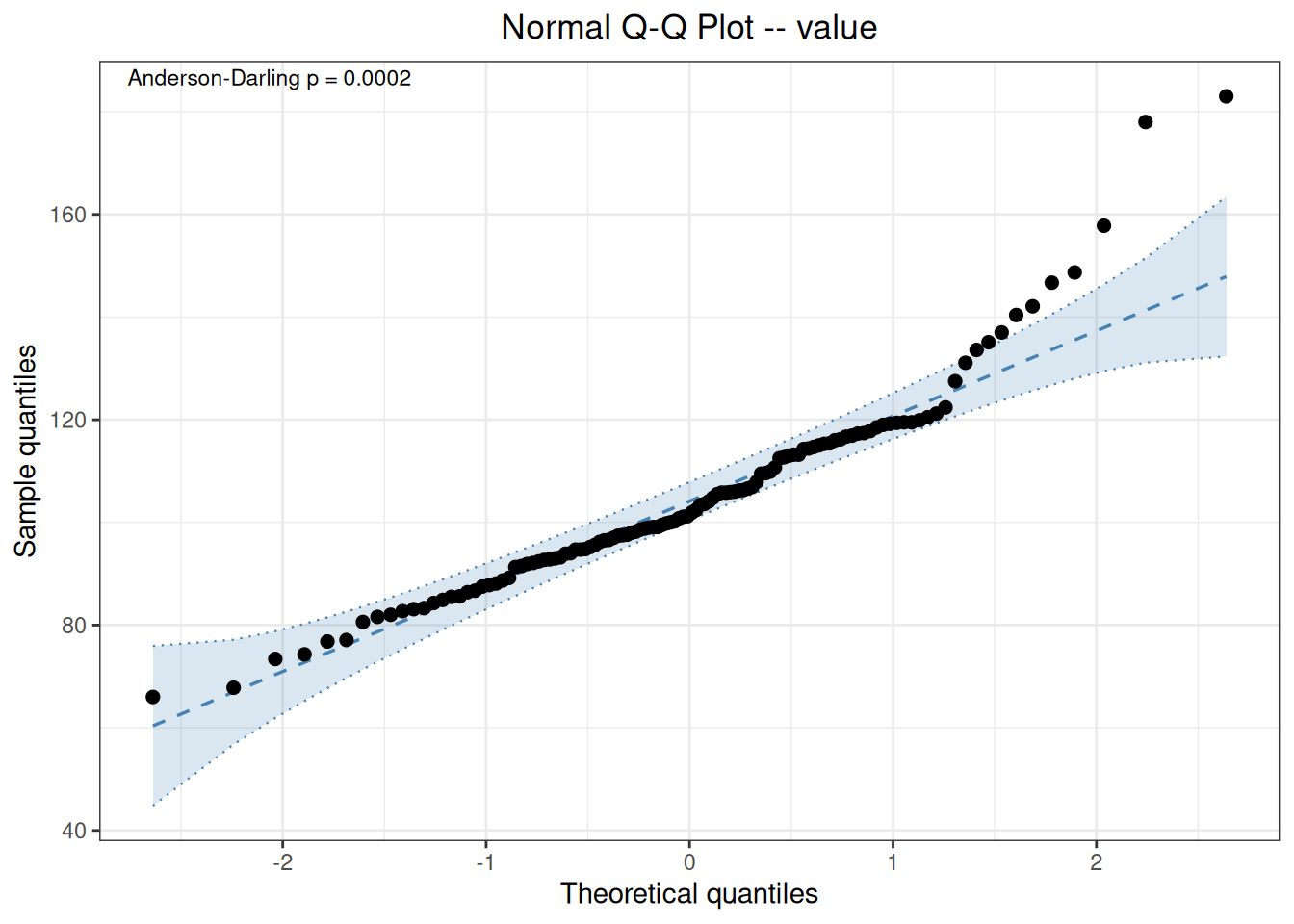
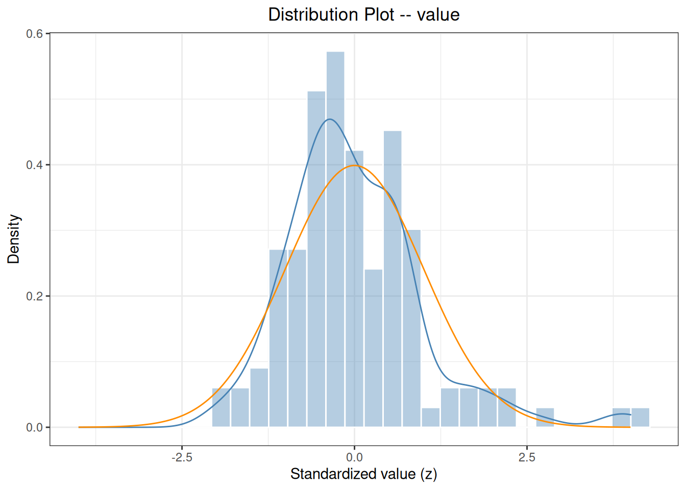
method="auto" 对 n=120 自动选择 Anderson-Darling 检验,p 值很小,提示数据不服从正态分布(该数据右偏并含离群值)。QQ 图与直方图可直观确认偏态。
代码
set.seed(1728)
ri <- reference_interval(
  ri_data,
  col = "value",
  interval = 0.95,
  ci = 0.95,
  method = "all",
  id = "id",
  bootstrap_replicates = 1999,
  seed = 1728
)
print(ri)
Reference Interval Analysis
  Column:              value
  Reference interval:  95% (alpha = 0.025)
  Confidence level:    0.95
  ID variable:         id
  Complete cases:      120 / 120

  No missing values.
  No duplicate IDs found.

  Nonparametric (CLSI EP28-A3c; exact binomial rank CI)
    Lower = 73.4225  [66.0000, 81.6000]
    Upper = 157.5725  [137.0000, 183.0000]
    Point ranks: 3.0250 and 117.9750
    CI ranks: lower 1-8; upper 113-120
    Actual rank coverage: lower 0.9412; upper 0.9412
    Warning: requested rank-CI coverage is not fully attainable at this sample size.

  Biweight (CLSI EP28-A3c Appendix B; 6 iterations)
    Lower = 63.2548  [54.4269, 71.4132]
    Upper = 141.7011  [133.3354, 149.8618]
    Tbi = 102.477938; sbi[205.6] = 19.748969; ST[3.7] = 1.536778
    Bootstrap valid: 1999 / 1999

  Type 6 (R quantile type 6; normal-approximation rank CI)
    Lower = 73.4225  [66.0000, 80.6000]
    Upper = 157.5725  [137.0000, 183.0000]

  Parametric (log-transformed, Shapiro-Wilk p = 0.0661)
    Lower = 73.2539  [69.3807, 77.3434]
    Upper = 145.9407  [138.2241, 154.0880]

  Huber (Huber M-estimation (k=1.5, 16 iter) + MAD)
    Lower = 72.1573  [66.8868, 77.1452]
    Upper = 134.7365  [128.8693, 142.7196]
    Bootstrap valid: 1999 / 1999
代码
plot(ri)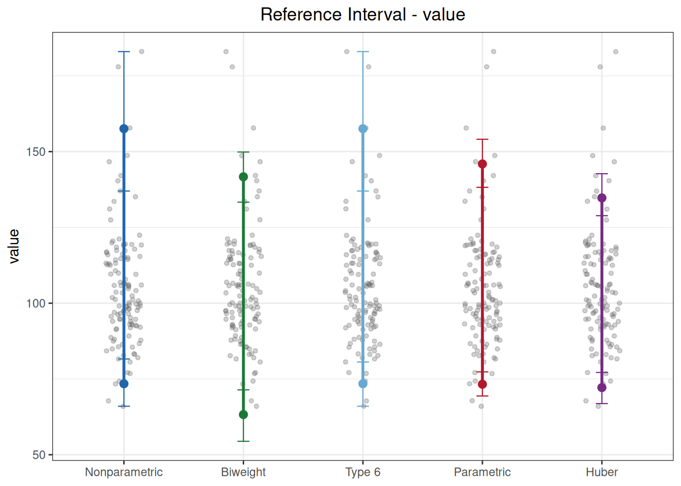
reference_interval() 中 interval 是参考区间覆盖度(默认 0.95,对应 2.5%–97.5%),ci 是区间端点的置信水平,两者含义不同。method 可取 "nonparametric"、"biweight"、"type6"、"parametric"、"huber" 的任意组合,或单独使用 "all"。id 用于重复样本检测。
本示例五种方法结果比较:
- 非参数法(73.4–157.6):EP28 点估计不作分布假设,端点 CI 使用二项秩;
- biweight 法(63.3–141.7):使用 EP28 附录 B 的两个尺度分量;该含离群值教学数据并未满足“先调查异常值”的前提;
- type-6 法(73.4–157.6):点估计与非参数法相同,但端点 CI 使用保留的正态近似秩;
- 参数法(73.3–145.9):自动检测到数据非正态后做了 log 变换(
transformed=TRUE)再回代; - Huber 法(72.2–134.7):基于 Huber M 估计与 MAD。
方法间差异反映了秩区间、分布假设和稳健尺度定义的不同。
17.2.2 标准案例:CLSI EP28-A3c 附录 B 稳健法迭代
附录 B 用女性钙数据中的 20 个观测演示 biweight 计算。该小样本仅为算法展示,标准明确不建议据此建立正式参考区间。method="biweight" 直接返回附录 B 的位置、尺度分量、参考限和 bootstrap 端点区间。
代码
ep28_b <- as.data.frame(read_csv(
  "./data/017-参考区间/std-ep28-appendix-b.csv",
  show_col_types = FALSE
))
ep28_biweight <- reference_interval(
  ep28_b, col = "calcium", interval = 0.95,
  ci = 0.90, method = "biweight",
  bootstrap_replicates = 1999, seed = 2803
)
ep28_biweight
Reference Interval Analysis
  Column:              calcium
  Reference interval:  95% (alpha = 0.025)
  Confidence level:    0.9
  ID variable:         --
  Complete cases:      20 / 20

  No missing values.
  Note: 'id' not provided, skip duplicate detection.

  Biweight (CLSI EP28-A3c Appendix B; 6 iterations)
    Lower = 9.0495  [8.8339, 9.2781]
    Upper = 10.1994  [9.9725, 10.4052]
    Tbi = 9.624439; sbi[205.6] = 0.270427; ST[3.7] = 0.048187
Bootstrap valid: 1989 / 1999| 标准位置 | 统计量 | 标准结果 | ivdtools结果 |
|---|---|---|---|
| EP28-A3c Appendix B | Tbi | 9.62440 | 9.62444 |
| EP28-A3c Appendix B | sbi[205.6] | 0.27043 | 0.27043 |
| EP28-A3c Appendix B | ST[3.7] | 0.04816 | 0.04819 |
| EP28-A3c Appendix B | lower | 9.05000 | 9.04951 |
| EP28-A3c Appendix B | upper | 10.20000 | 10.19937 |
\(S_T\) 未舍入值与标准显示值相差约 \(2.7\times10^{-5}\),属于标准中间量舍入差异,表中如实保留。正式参考区间仍应使用满足方案要求的样本;标准明确指出 20 点数据只用于展示算法,而且稳健法也要求先调查并处理有依据的异常观测。