%%{init: {"theme":"base","themeVariables":{"primaryColor":"#EAF2FB","primaryBorderColor":"#2780E3","primaryTextColor":"#212529","lineColor":"#6C757D","secondaryColor":"#EAF7E6","tertiaryColor":"#FFF4E8","fontSize":"13px"},"flowchart":{"nodeSpacing":18,"rankSpacing":24,"padding":6}}}%%

flowchart LR
    A{"输入数据层级"} -->|逐例判定| B["raw_to_table()"]
    A -->|TP/FP/TN/FN| C["counts_to_table()"]
    B --> D["diagnostics() / kappa()<br/>mcnemar()"]
    C --> D
    A -->|连续内部响应| E["continuous_to_binary()<br/>或 c5_c95()"]
    D --> F["临床性能或<br/>观察者一致性"]
    E --> G["阈值附近检出概率<br/>或声明验证"]

    classDef input fill:#EAF2FB,stroke:#2780E3,color:#212529
    classDef process fill:#EAF7E6,stroke:#3FB618,color:#212529
    classDef decision fill:#FFF4E8,stroke:#FF7518,color:#212529
    classDef output fill:#F4EEFB,stroke:#9954BB,color:#212529
    class A decision
    class B,C,D,E process
    class F,G output
15 定性分析与 C5/C95
本文回答三个层次不同的问题:候选方法与参考方法的二分类结果是否一致、阳性/阴性判定的一致程度有多大,以及连续响应在临界浓度附近达到指定检出概率的位置。前两类问题使用配对四格表,后一类问题使用 c5_c95()。
重要使用边界
分析前必须固定阳性方向、参考方法或临床状态定义、重复测量的合并规则和置信区间方法。若一个受试者有多次结果,应先按方案确定“受试者级”判定,不能把重复结果直接当作独立样本扩大样本量。
分析流程:从判定结果到定性性能结论
定性(qualitative)分析评价候选方法与参考方法在阳性/阴性判定上的一致程度,对应 CLSI EP12。ivdtools 提供 raw_to_table() 从原始配对数据构建四格表,counts_to_table() 从已有的 TP/FP/TN/FN 计数直接构建,并配套 diagnostics()(灵敏度、特异度、PPV、NPV、似然比等)、kappa()(Kappa 与 PABAK)与 mcnemar()(配对差异检验)三个分析方法。定量结果需转定性时可用 continuous_to_binary()。
代码
library(ivdtools)
library(readr)
15.1 主要函数
| 函数 | 主要用途 | 关键输入或输出 |
|---|---|---|
raw_to_table() |
原始配对数据构建四格表 | candidate、reference、 positive、 na.rm |
counts_to_table() |
由 TP/FP/TN/FN 构建四格表 | candidate/reference 命名 |
continuous_to_binary() |
定量转定性 | cutoff(≥ cutoff 为 1) |
describe() |
原始数据描述 | 仅 raw_to_table() 来源可用 |
diagnostics() |
诊断准确性指标 | ci.method、prevalence |
kappa() |
Kappa / PABAK | prevalence 切换 |
mcnemar() |
配对差异检验 | 不一致对 <25 用精确检验 |
c5_c95() |
内部连续响应的 C5/C95 | cutoff、direction、精密度剖面 |
选择函数时,先看数据处于哪一个层级:已有 TP/FP/TN/FN 时使用 counts_to_table();有逐受试者配对判定时使用 raw_to_table();只有连续信号和参考浓度时,先确认能否建立 c5_c95() 所需的重复性/精密度关系。diagnostics()、kappa() 和 mcnemar() 的统计对象都来自同一张四格表,报告时应保持分母一致。
15.1.1 四格表指标与检验公式
代码
raw_to_table(data, candidate, reference, id = NULL,
             na.rm = TRUE, positive = NULL)
counts_to_table(tp, fp, tn, fn,
                candidate = "candidate", reference = "reference")
diagnostics(object, conf.level = 0.95,
            ci.method = "wilson", prevalence = NULL)
kappa(x, prevalence = NULL, conf.level = 0.95)
mcnemar(x, conf.level = 0.95)
约定四格表为 \(a=TP,b=FP,c=FN,d=TN\)。主要指标为
\[ Se=\frac{a}{a+c},\quad Sp=\frac{d}{b+d},\quad PPV=\frac{a}{a+b},\quad NPV=\frac{d}{c+d}, \]
\[ LR^+=\frac{Se}{1-Sp},\qquad LR^-=\frac{1-Se}{Sp}. \]
diagnostics() 的比例区间可选 Wilson、Wald、连续性校正 Wald/Wilson、Agresti–Coull、Jeffreys 或 Clopper–Pearson。给出目标人群患病率 \(\pi\) 时,PPV/NPV 用贝叶斯关系重算;其余指标仍来自原四格表。零格时 LR 或 OR 的对数近似区间可能为 NA,函数不自动作 0.5 校正。
Cohen Kappa 使用
\[ \kappa=\frac{P_o-P_e}{1-P_e},\qquad P_o=\frac{a+d}{n}, \]
其中 \(P_e\) 由两种判定的边际比例计算。向 kappa() 传入 prevalence 时,当前实现切换为 \(PABAK=2P_o-1\);该数值参数只触发 PABAK 并记录标签,不进入公式。McNemar 只使用不一致对 \(b,c\):\(b+c<25\) 时做双侧精确二项检验,否则使用连续性校正统计量
\[ \chi^2=\frac{(|b-c|-1)^2}{b+c}. \]
raw_to_table() 和 counts_to_table() 返回四格表对象;continuous_to_binary() 返回新增二分类列的数据框;describe() 返回描述统计表;diagnostics()、kappa() 和 mcnemar() 返回统计量、区间和检验结果
15.1.2 C5/C95 的概率模型
代码
c5_c95(data, result = NULL, sample = NULL, cutoff,
       direction = c("geq", "leq"),
       probabilities = c(0.05, 0.95), component = NULL,
       model.no = 1:10, K = 2, search_range = NULL)
对内部连续响应均值 \(\mu\) 和精密度轮廓 \(\sigma(\mu)\),direction="geq" 时
\[ P(\text{阳性}\mid\mu) =1-\Phi\left(\frac{c-\mu}{\sigma(\mu)}\right). \]
C5/C95 是分别令该概率等于 0.05 和 0.95 时求得的 \(\mu\)。输入可为原始重复数据,也可为已经执行 variance() 的 precision 对象。若存在多个根,函数选取最接近 cutoff 的根;无根、多根或超出观测均值范围都会记录在 issues,不应静默忽略。
c5_c95() 返回 C5/C95、拟合模型和 issues。
15.2 分析案例
15.2.1 示例一:原始配对数据的完整分析
代码
qual <- read_csv("./data/015-定性分析与C5C95/qualitative-raw.csv", show_col_types = FALSE)
qual <- as.data.frame(qual)

qa <- raw_to_table(
  qual,
  candidate = "new",
  reference = "gold",
  id = "id",
  positive = "positive"
)
qa
Fourfold Table
  Source            : raw data
  Total n           : 60
  Duplicate IDs     : none
  Candidate         : new
  Reference         : gold

  2x2 Contingency Table
  ----------------------------------------
              gold
                  positive  negative  Sum
  ----------------------------------------
  new   positive  23        1         24
        negative  1         35        36
        sum       24        36        60
  ----------------------------------------
raw_to_table() 要求候选与参考列都恰好有 2 个水平;positive 指定阳性水平(用于因子/字符列的水平映射);na.rm 控制是否删除缺失行。id 可选,用于重复样本检测。
代码
qa <- describe(qa)
Data Summary
  Rows:    60
  Columns: 5
  ID:      60 unique, no duplicates

  new
    negative        36  ( 60.0%)
    positive        24  ( 40.0%)
  gold
    negative        36  ( 60.0%)
    positive        24  ( 40.0%)
  age
    Mean (SD):       51.05 (13.45)
    Median (Q1-Q3):  48.90 (42.15 - 57.28)
    Range:           24.30 - 90.10
  gender
    F               32  ( 53.3%)
    M               28  ( 46.7%)
describe() 仅对 raw_to_table() 来源可用,输出行数、ID 重复、各列摘要与缺失情况。
代码
qa <- diagnostics(qa, ci.method = "wilson")
Diagnostic Performance Summary
  Sensitivity        0.958  (0.798, 0.993)
  Specificity        0.972  (0.858, 0.995)
  PPV                0.958  (0.798, 0.993)
  NPV                0.972  (0.858, 0.995)
  Accuracy           0.967  (0.886, 0.991)
  Prevalence         0.400  (0.286, 0.526)
  LR+                34.500  (4.986, 238.724)
  LR-                0.043  (0.006, 0.292)
  Odds Ratio         805.000  (47.921, 13522.837)

  # PPV & NPV are based on data prevalence of 0.400.
  # Confidence intervals for proportions use 'wilson' method.
本例灵敏度 0.958、特异度 0.972。若已知目标人群患病率,可用 prevalence 重算 PPV/NPV:
代码
qa <- diagnostics(qa, prevalence = 0.4)
Diagnostic Performance Summary
  Sensitivity        0.958  (0.798, 0.993)
  Specificity        0.972  (0.858, 0.995)
  PPV                0.958  (0.790, 0.993)
  NPV                0.972  (0.864, 0.995)
  Accuracy           0.967  (0.886, 0.991)
  Prevalence         0.400
  LR+                34.500  (4.986, 238.724)
  LR-                0.043  (0.006, 0.292)
  Odds Ratio         805.000  (47.921, 13522.837)

  # PPV & NPV are based on user-specified prevalence of 0.400.
  # Confidence intervals for proportions use 'wilson' method.
diagnostics() 的 ci.method 可选 7 种比例置信区间方法(默认 "wilson");给出 prevalence 时 PPV/NPV 按贝叶斯公式重算,否则基于数据患病率。
代码
qa <- kappa(qa)
Cohen's Kappa
  new  vs  gold
  n = 60

  Kappa                 0.9306
  SE                    0.0483
  95% CI                (0.8359, 1.0000)
  Observed agreement    0.9667
  Expected agreement    0.5200
代码
qa <- kappa(qa, prevalence = 0.5)
PABAK
  new  vs  gold
  n = 60

  Kappa                 0.9333
  SE                    0.0463
  95% CI                (0.8425, 1.0000)
  Observed agreement    0.9667
  Expected agreement    0.5000
  # PABAK (prevalence = 0.500): 2 * p_obs - 1, assumes expected agreement = 0.5
kappa() 给出 Cohen’s Kappa;当给出 prevalence 时改为计算 PABAK(2·p_obs − 1)。两者对患病率偏倚的处理不同,报告时应注明方法。
代码
qa <- mcnemar(qa)
McNemar Test
  new  vs  gold
  Discordant pairs:  b (pos, neg) = 1,  c (neg, pos) = 1
  n (b + c)        = 2

  Method: Exact binomial test
  P-value:          1.0000
  Conclusion: Not significant at 95% confidence level
不一致对 b+c = 2 < 25,函数自动使用精确二项检验。
代码
summary(qa)
Qualitative Analysis - summary
-------------------------------------------------

Fourfold Table
  Source            : raw data
  Total n           : 60
  Duplicate IDs     : none
  Candidate         : new
  Reference         : gold

  2x2 Contingency Table
  ----------------------------------------
              gold
                  positive  negative  Sum
  ----------------------------------------
  new   positive  23        1         24
        negative  1         35        36
        sum       24        36        60
  ----------------------------------------

Analyses performed:

  [x] Describe
  [x] Diagnostics
  [x] Kappa
  [x] McNemar

Data Summary
  Rows:    60
  Columns: 5
  ID:      60 unique, no duplicates

  new
    negative        36  ( 60.0%)
    positive        24  ( 40.0%)
  gold
    negative        36  ( 60.0%)
    positive        24  ( 40.0%)
  age
    Mean (SD):       51.05 (13.45)
    Median (Q1-Q3):  48.90 (42.15 - 57.28)
    Range:           24.30 - 90.10
  gender
    F               32  ( 53.3%)
    M               28  ( 46.7%)

Diagnostic Performance Summary
  Sensitivity        0.958  (0.798, 0.993)
  Specificity        0.972  (0.858, 0.995)
  PPV                0.958  (0.790, 0.993)
  NPV                0.972  (0.864, 0.995)
  Accuracy           0.967  (0.886, 0.991)
  Prevalence         0.400
  LR+                34.500  (4.986, 238.724)
  LR-                0.043  (0.006, 0.292)
  Odds Ratio         805.000  (47.921, 13522.837)

  # PPV & NPV are based on user-specified prevalence of 0.400.
  # Confidence intervals for proportions use 'wilson' method.

PABAK
  new  vs  gold
  n = 60

  Kappa                 0.9333
  SE                    0.0463
  95% CI                (0.8425, 1.0000)
  Observed agreement    0.9667
  Expected agreement    0.5000
  # PABAK (prevalence = 0.500): 2 * p_obs - 1, assumes expected agreement = 0.5

McNemar Test
  new  vs  gold
  Discordant pairs:  b (pos, neg) = 1,  c (neg, pos) = 1
  n (b + c)        = 2

  Method: Exact binomial test
  P-value:          1.0000
  Conclusion: Not significant at 95% confidence level
15.2.2 示例二:由 TP/FP/TN/FN 直接构建
代码
tab <- counts_to_table(
  tp = 80, fp = 5, tn = 120, fn = 3,
  candidate = "new method",
  reference = "gold standard"
)
tab
Fourfold Table
  Source            : counts
  Total n           : 208
  Candidate         : new method
  Reference         : gold standard

  2x2 Contingency Table
  -----------------------------------------------
                     gold standard
                         positive  negative  Sum
  -----------------------------------------------
  new method   positive  80        5         85
               negative  3         120       123
               sum       83        125       208
  -----------------------------------------------
代码
tab <- diagnostics(tab)
Diagnostic Performance Summary
  Sensitivity        0.964  (0.899, 0.988)
  Specificity        0.960  (0.910, 0.983)
  PPV                0.941  (0.870, 0.975)
  NPV                0.976  (0.931, 0.992)
  Accuracy           0.962  (0.926, 0.980)
  Prevalence         0.399  (0.335, 0.467)
  LR+                24.096  (10.198, 56.934)
  LR-                0.038  (0.012, 0.114)
  Odds Ratio         640.000  (148.773, 2753.180)

  # PPV & NPV are based on data prevalence of 0.399.
  # Confidence intervals for proportions use 'wilson' method.
代码
tab <- kappa(tab)
Cohen's Kappa
  new method  vs  gold standard
  n = 208

  Kappa                 0.9201
  SE                    0.0277
  95% CI                (0.8659, 0.9744)
  Observed agreement    0.9615
  Expected agreement    0.5184
代码
tab <- mcnemar(tab)
McNemar Test
  new method  vs  gold standard
  Discordant pairs:  b (pos, neg) = 5,  c (neg, pos) = 3
  n (b + c)        = 8

  Method: Exact binomial test
  P-value:          0.7266
  Conclusion: Not significant at 95% confidence level
代码
describe(tab) # counts 来源无原始数据,describe() 不可用counts_to_table() 构建的对象没有原始数据,因此 describe() 不可用;diagnostics()、kappa()、 mcnemar() 均正常。
15.2.3 示例三:定量数据转定性
候选方法为定量结果 result,参考为定性 gold:
代码
cont <- read_csv("./data/015-定性分析与C5C95/qualitative-continuous.csv", show_col_types = FALSE)
cont <- as.data.frame(cont)
head(cont, 6)
id result gold
1 S001 10.111087 positive
2 S002 13.057209 positive
3 S003 1.534680 negative
4 S004 7.782787 negative
5 S005 4.982424 negative
6 S006 9.443399 negative按 cutoff = 8 转二分类:
代码
cont_bin <- continuous_to_binary(cont, cols = "result", cutoff = 8)
head(cont_bin, 6)
id result gold result_binary
1 S001 10.111087 positive 1
2 S002 13.057209 positive 1
3 S003 1.534680 negative 0
4 S004 7.782787 negative 0
5 S005 4.982424 negative 0
6 S006 9.443399 negative 1continuous_to_binary() 生成 result_binary 列(≥ cutoff 为 1,否则 0)。为满足 raw_to_table() 的 positive 映射要求,先重标为与参考一致的标签:
代码
cont_bin$result_binary_lab <- ifelse(cont_bin$result_binary == 1, "positive", "negative")代码
qa3 <- raw_to_table(
  cont_bin,
  candidate = "result_binary_lab",
  reference = "gold",
  id = "id",
  positive = "positive"
)
qa3 <- diagnostics(qa3)
Diagnostic Performance Summary
  Sensitivity        0.952  (0.773, 0.992)
  Specificity        0.897  (0.736, 0.964)
  PPV                0.870  (0.679, 0.955)
  NPV                0.963  (0.817, 0.993)
  Accuracy           0.920  (0.812, 0.968)
  Prevalence         0.420  (0.294, 0.558)
  LR+                9.206  (3.140, 26.994)
  LR-                0.053  (0.008, 0.361)
  Odds Ratio         173.333  (16.746, 1794.100)

  # PPV & NPV are based on data prevalence of 0.420.
  # Confidence intervals for proportions use 'wilson' method.
positive 指定的水平必须同时存在于两列中,因此先把二值列重标为 positive/negative。若不指定 positive,函数可能按排序水平把阳性/阴性方向颠倒,导致 TP/FP 翻转,务必核对。
15.2.4 示例四:由内部连续响应估计 C5/C95
当定性判定来自内部连续信号与固定 cutoff 时,可用重复测量建立 SD-均值精密度剖面,再求达到指定阳性概率时的平均响应。下面以 result >= 40 定义目标事件:
代码
head(c5_data, 6) level response
1 L1 35.14000
2 L1 35.29636
3 L1 35.45273
4 L1 35.60909
5 L1 35.76545
6 L1 35.92182代码
c5_result <- c5_c95(
  c5_data,
  result = "response",
  sample = "level",
  cutoff = 40,
  direction = "geq",
  probabilities = c(0.05, 0.95),
  model.no = 1
)
c5_result
C5/C95 estimation from an internal continuous response
Source: raw data
Precision component: repeatability
Event: response >= cutoff
cutoff label probability mean_response SD actual_probability extrapolated
------------------------------------------------------------------------------
40 C5 0.05 39.0291 0.5903 0.05 FALSE
40 C95 0.95 40.9709 0.5903 0.95 FALSE 代码
plot(c5_result, type = "probability")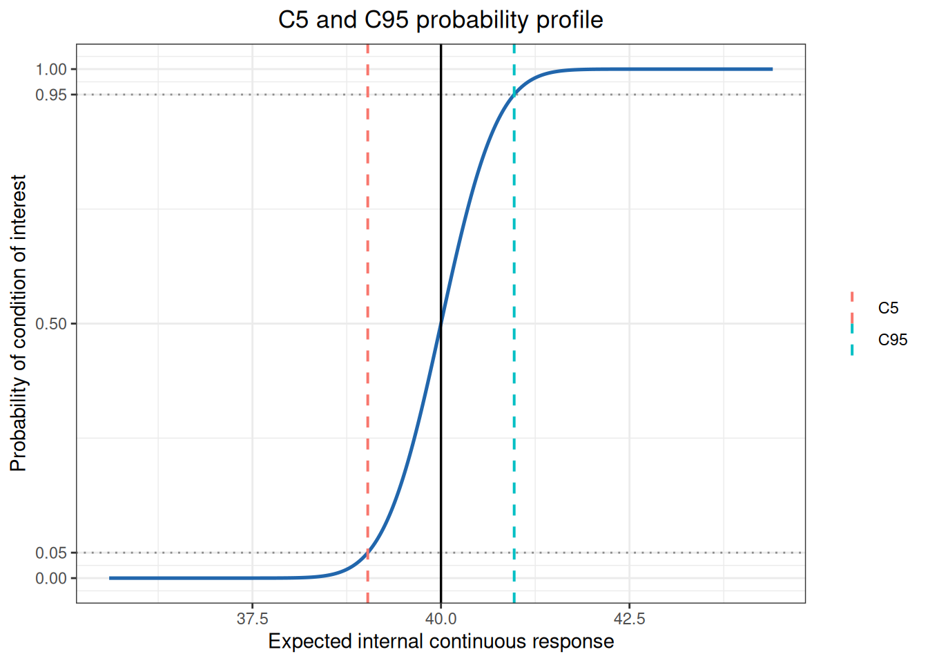
direction = "geq" 表示响应大于等于 cutoff 为目标事件,"leq" 表示小于等于 cutoff。若根超出实测均值范围,对象会标记外推;精密度剖面的模型选择与覆盖范围应纳入结果解释。