%%{init: {"theme":"base","themeVariables":{"primaryColor":"#EAF2FB","primaryBorderColor":"#2780E3","primaryTextColor":"#212529","lineColor":"#6C757D","secondaryColor":"#EAF7E6","tertiaryColor":"#FFF4E8","fontSize":"13px"},"flowchart":{"nodeSpacing":18,"rankSpacing":24,"padding":6}}}%%

flowchart LR
    A["重复、证书、IQC<br/>均匀性、稳定性、定值"]
    B["各 uncertainty_*() 函数<br/>转换为标准不确定度分量"]
    C["uncertainty_combine()<br/>单节点预算"]
    D["uncertainty_propagate()<br/>测量模型传播"]
    E["uncertainty_traceability()<br/>逐级溯源预算"]

    A --> B
    B --> C
    B --> D --> C
    C --> E

    classDef source fill:#EAF2FB,stroke:#2780E3,color:#212529
    classDef function fill:#EAF7E6,stroke:#3FB618,color:#212529
    classDef result fill:#F4EEFB,stroke:#9954BB,color:#212529

    class A source
    class B,C,D function
    class E result
5 不确定度分析
本文演示如何使用 ivdtools 包建立测量不确定度分量、传播测量模型、合成不确定度预算,并沿计量溯源阶段汇总结果。内容覆盖 A 类和 B 类评价、长期 IQC、瓶间均匀性、稳定性、多实验室定值以及单节点和逐级预算。
重要使用边界
本文中的普通数据和标准案例数据仅用于验证分析流程。uncertainty_* 系列函数计算标准不确定度、合成不确定度和扩展不确定度,不替代被测量定义、实验设计、临床接受标准、法规评价或产品放行结论。正式报告必须说明被测量、单位、结果是单次值还是均值、各分量的来源、分布、自由度、覆盖因子和相关性假设。
标准案例的数值以标准原文为依据;每个案例均将 ivdtools 计算结果与标准原文结果逐项比较。标准原文的中间舍入、统计口径或近似方法与函数默认计算不同而产生的差异,会在对照表后单独说明。
测量不确定度分析首先明确输出量和测量模型,再把不同来源的信息转换为标准不确定度分量:
设输入量的标准不确定度为 \(u_i\),灵敏度系数为 \(c_i\),则在独立假设下,合成标准不确定度可表示为:
\[u_c = \sqrt{\sum_i (c_i u_i)^2}\]
有相关性时还应加入协方差项。扩展不确定度为:
\[U = k u_c\]
其中 \(k\) 为覆盖因子。relative = TRUE 保存相对标准不确定度;相对分量和绝对分量混合时,应向 uncertainty_combine() 提供结果量值 value。
代码
library(ivdtools)
library(readr)
5.1 主要函数
| 函数 | 主要用途 |
|---|---|
| uncertainty_type_a() | 由重复测量估计 A 类分量 |
| uncertainty_type_b() | 由证书、上下限或分布估计 B 类分量 |
| uncertainty_iqc() | 从长期 IQC 提取批内、批间和综合分量 |
| uncertainty_homogeneity() | 评价瓶间或单元间均匀性 |
| uncertainty_stability() | 由时间趋势估计货架期稳定性分量 |
| uncertainty_characterization() | 由多实验室结果估计定值分量 |
| uncertainty_combine() | 合成一个结果节点的不确定度预算 |
| uncertainty_propagate() | 传播除法、乘法或其他测量模型 |
| uncertainty_traceability() | 沿溯源阶段逐级累计新增分量 |
5.1.1 重复测量的 A 类分量 uncertainty_type_a()
quantity = “single” 使用重复结果的样本标准差,描述未来单次结果;quantity = “mean” 使用标准误,描述这组重复结果的均值。二者对应的被报告量不同。
代码
repeatability <- uncertainty_type_a(
  c(99.5, 100.2, 100.0, 99.8, 100.1),
  name = "重复测量",
  quantity = "mean",
  relative = TRUE
)

repeatability
Uncertainty component
  Name                 : 重复测量
  Estimate             : 99.92
  Standard uncertainty : 0.0012419609
  Relative uncertainty : 0.0012419609
  Degrees of freedom   : 4
  Evaluation type      : A
  Distribution         : normal
  Source               : replicate measurements: mean
  Relative             : TRUE
返回对象包含估计值、标准不确定度、相对标准不确定度、自由度、评价类型、分布和来源等字段。非有限值会被排除,但正式分析仍应保存原始数据和排除记录。
5.1.2 证书或规格的 B 类分量 uncertainty_type_b()
当证书直接给出扩展不确定度时,必须提供证书对应的 k;当只有上下限时,应根据证书、规格或科学依据选择分布。
代码
certificate <- uncertainty_type_b(
  name = "校准品证书",
  estimate = 100,
  uncertainty = 2,
  distribution = "normal",
  k = 2,
  relative = TRUE
)

pipette <- uncertainty_type_b(
  name = "移液器容量",
  estimate = 10,
  lower = 9.9,
  upper = 10.1,
  distribution = "rectangular"
)

certificate
Uncertainty component
  Name                 : 校准品证书
  Estimate             : 100
  Standard uncertainty : 0.01
  Relative uncertainty : 0.01
  Degrees of freedom   : Inf
  Evaluation type      : B
  Distribution         : normal
  Source               : expanded uncertainty
  Relative             : TRUE
代码
pipette
Uncertainty component
  Name                 : 移液器容量
  Estimate             : 10
  Standard uncertainty : 0.057735027
  Relative uncertainty : 0.0057735027
  Degrees of freedom   : Inf
  Evaluation type      : B
  Distribution         : rectangular
  Source               : interval limits
  Relative             : FALSE
区间分布的标准不确定度由区间半宽和分布假设共同决定。正态或 Student t 区间还需要明确覆盖概率和自由度。
5.1.3 长期 IQC 分量 uncertainty_iqc()
有运行批次和批内重复时,函数使用单因素随机效应 ANOVA 分解批内和批间变异;没有 run 列或每个运行只有一个结果时,直接使用长期结果的离散程度。
代码
iqc_data <- data.frame(
  run = rep(1:5, each = 2),
  result = c(99, 101, 100, 102, 98, 100, 101, 103, 99, 100)
)

iqc_component <- uncertainty_iqc(
  iqc_data,
  result = "result",
  run = "run",
  quantity = "single",
  name = "长期 IQC",
  relative = TRUE
)

iqc_component
IQC uncertainty
  Method                    : one-way ANOVA
  Observations              : 10
  Runs                      : 5
  Within-run SD             : 1.3038405
  Between-run SD            : 0.77459667
  Single-result uncertainty : 1.5165751
  Mean uncertainty          : 0.53851648
IQC 水平应代表被报告结果的浓度水平。失控期间是否排除必须由预先规定的质量程序决定;如果 IQC 已包含某个校准或批间来源,不应把相同来源再次作为独立分量加入。
5.1.4 瓶间均匀性分量 uncertainty_homogeneity()
数据应为长格式,每个包装单元通常包含多次重复测量。函数返回均方、重复性标准差、观察到的单元间标准差、隐含不均匀性和最终的 u_bb。
代码
homogeneity_data <- data.frame(
  bottle = rep(paste0("B", 1:4), each = 2),
  result = c(99, 100, 101, 100, 98, 99, 102, 101)
)

homogeneity_component <- uncertainty_homogeneity(
  homogeneity_data,
  unit = "bottle",
  result = "result",
  name = "瓶间均匀性",
  relative = TRUE
)

homogeneity_component
Between-unit homogeneity uncertainty
  Units                             : 4
  Results                           : 8
  Mean                              : 100
  Effective degrees of freedom      : 2
  Average replicates                : 2
  Within-unit mean square           : 0.5
  Between-unit mean square          : 3.3333333
  Within-unit degrees of freedom    : 4
  Between-unit degrees of freedom   : 3
  Repeatability SD                  : 0.70710678
  Between-unit SD                   : 1.1902381
  Hidden inhomogeneity              : 0.42044821
  Between-unit uncertainty          : 1.1902381
  Relative repeatability            : 0.0070710678
  Relative between-unit             : 0.011902381
  Relative hidden inhomogeneity     : 0.0042044821
  Relative between-unit uncertainty : 0.011902381
均匀性结果还取决于抽样方式、测量顺序和最小取样量。函数不会自动证明取样方案足以代表整批产品。
5.1.5 稳定性趋势分量 uncertainty_stability()
函数拟合:
\[result = intercept + slope \times time\]
目标货架期上的趋势不确定度为斜率标准误乘以货架期。shelf_life 与 time 必须使用同一时间单位。
代码
stability_data <- data.frame(
  time = rep(0:4, each = 2),
  result = c(100.1, 99.9, 100.0, 99.8, 99.7,
             99.9, 99.6, 99.8, 99.5, 99.7)
)

stability_component <- uncertainty_stability(
  stability_data,
  time = "time",
  result = "result",
  shelf_life = 6,
  name = "6个月长期稳定性",
  relative = TRUE
)

stability_component
Stability uncertainty
  Condition                      : all
  Observations                   : 10
  Minimum time                   : 0
  Maximum time                   : 4
  Shelf life                     : 6
  Intercept                      : 100
  Slope                          : -0.1
  Mean                           : 99.8
  Slope SE                       : 0.025
  Residual SD                    : 0.1118034
  Degrees of freedom             : 8
  Long-term uncertainty          : 0.15
  Relative long-term uncertainty : 0.001503006
严重超出实际观察范围的外推需要单独论证。多个储存条件通常表示不同情景,不能不加判断地把所有条件的组件同时相加。
5.1.6 多实验室定值分量 uncertainty_characterization()
函数先计算每个实验室的均值,再对实验室均值等权汇总。某个实验室重复次数更多不会自动获得更大权重。
代码
characterization_data <- data.frame(
  laboratory = rep(paste0("Lab", 1:4), each = 3),
  result = c(
    99, 100, 101,
    100, 101, 100,
    98, 99, 100,
    101, 102, 101
  )
)

characterization_component <- uncertainty_characterization(
  characterization_data,
  laboratory = "laboratory",
  result = "result",
  name = "多实验室定值",
  relative = TRUE
)

characterization_component
Characterization uncertainty
  laboratories         : 4
  assigned_value       : 100.16667
  laboratory_sd        : 0.96225045
  standard_uncertainty : 0.48112522
5.1.7 单节点合成 uncertainty_combine()
uncertainty_combine() 适用于组件已经表达在同一输出尺度的情况。sensitivity 表示输入变化对输出的局部影响;correlation 用于提供输入量之间的相关矩阵。默认相关矩阵为单位矩阵,即假设分量相互独立。
代码
budget <- uncertainty_combine(
  repeatability,
  certificate,
  homogeneity_component$component,
  value = 100,
  coverage = 0.95,
  k = 2
)

budget
Combined uncertainty budget
  Scale: absolute
  Combined standard uncertainty: 1.55952
  Expanded uncertainty: 3.11903 (k = 2, 95.0%)

  Component: 重复测量
    Estimate                     : 99.92
    Standard uncertainty         : 0.0012419609
    Relative uncertainty         : 0.0012419609
    Degrees of freedom           : 4
    Evaluation type              : A
    Distribution                 : normal
    Source                       : replicate measurements: mean
    Relative                     : TRUE
    Sensitivity                  : 1
    Uncertainty on output scale  : 0.12419609
    Signed variance contribution : 0.01542467
    Contribution percent         : 0.63421424

  Component: 校准品证书
    Estimate                     : 100
    Standard uncertainty         : 0.01
    Relative uncertainty         : 0.01
    Degrees of freedom           : Inf
    Evaluation type              : B
    Distribution                 : normal
    Source                       : expanded uncertainty
    Relative                     : TRUE
    Sensitivity                  : 1
    Uncertainty on output scale  : 1
    Signed variance contribution : 1
    Contribution percent         : 41.116877

  Component: 瓶间均匀性
    Estimate                     : 100
    Standard uncertainty         : 0.011902381
    Relative uncertainty         : 0.011902381
    Degrees of freedom           : 3
    Evaluation type              : A
    Distribution                 : normal
    Source                       : EP30 homogeneity ANOVA
    Relative                     : TRUE
    Sensitivity                  : 1
    Uncertainty on output scale  : 1.1902381
    Signed variance contribution : 1.4166667
    Contribution percent         : 58.248909
预算对象还保存有效自由度、覆盖因子、协方差矩阵和各分量在输出尺度上的贡献。
代码
plot(budget)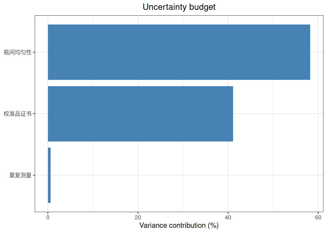
5.1.8 非线性测量模型 uncertainty_propagate()
对于比值、乘积、幂函数、对数或其他非线性测量模型,可用 uncertainty_propagate() 自动计算灵敏度并传播输入不确定度。组件名称必须与测量模型的形参名一致且唯一。
代码
mass <- uncertainty_type_b(
  "mass", estimate = 20, uncertainty = 0.2,
  distribution = "standard"
)
volume <- uncertainty_type_b(
  "volume", estimate = 4, uncertainty = 0.1,
  distribution = "standard"
)

concentration_delta <- uncertainty_propagate(
  model = function(mass, volume) mass / volume,
  components = list(mass, volume),
  method = "delta"
)
concentration_delta
Uncertainty propagation
  Method: delta
  Model estimate: 5
  Standard uncertainty: 0.134629
  95.0% interval: [4.73613, 5.26387]
代码
concentration_mc <- uncertainty_propagate(
  model = function(mass, volume) mass / volume,
  components = list(mass, volume),
  method = "monte_carlo",
  simulations = 10000,
  seed = 20260901
)
concentration_mc
Uncertainty propagation
  Method: monte_carlo
  Model estimate: 5
  Standard uncertainty: 0.13615
  95.0% interval: [4.75089, 5.28508]
delta 方法适合输入不确定度较小且模型在估计值附近近似线性的情况。Monte Carlo 可用于输出分布明显偏斜或需要非对称覆盖区间的场景;正式报告应保存模拟次数、随机种子、分布和相关结构。
代码
plot(concentration_delta, type = "contribution")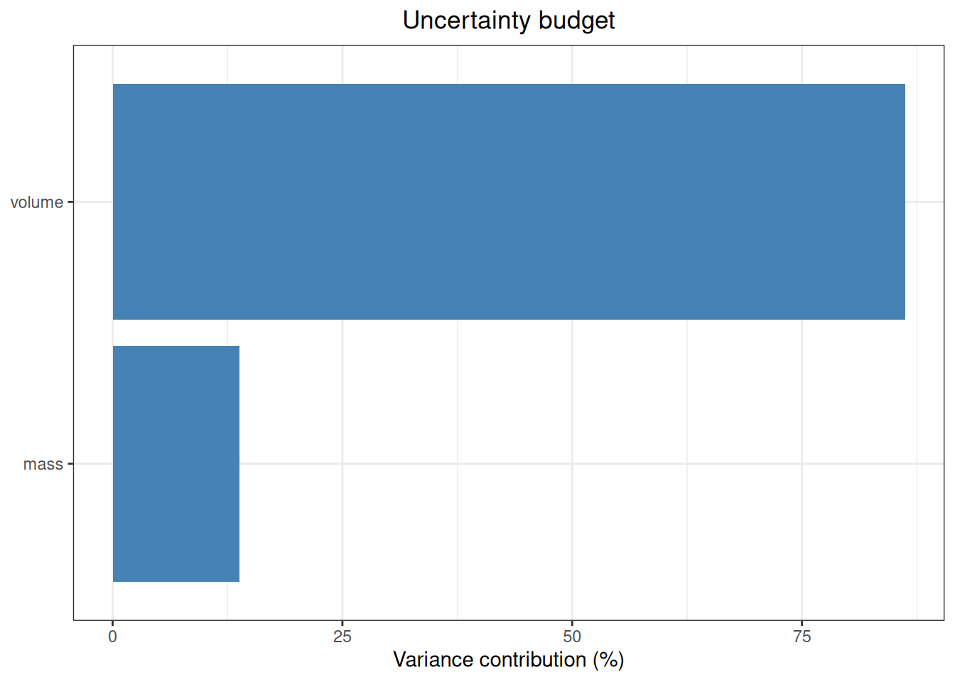
代码
plot(concentration_mc, type = "distribution")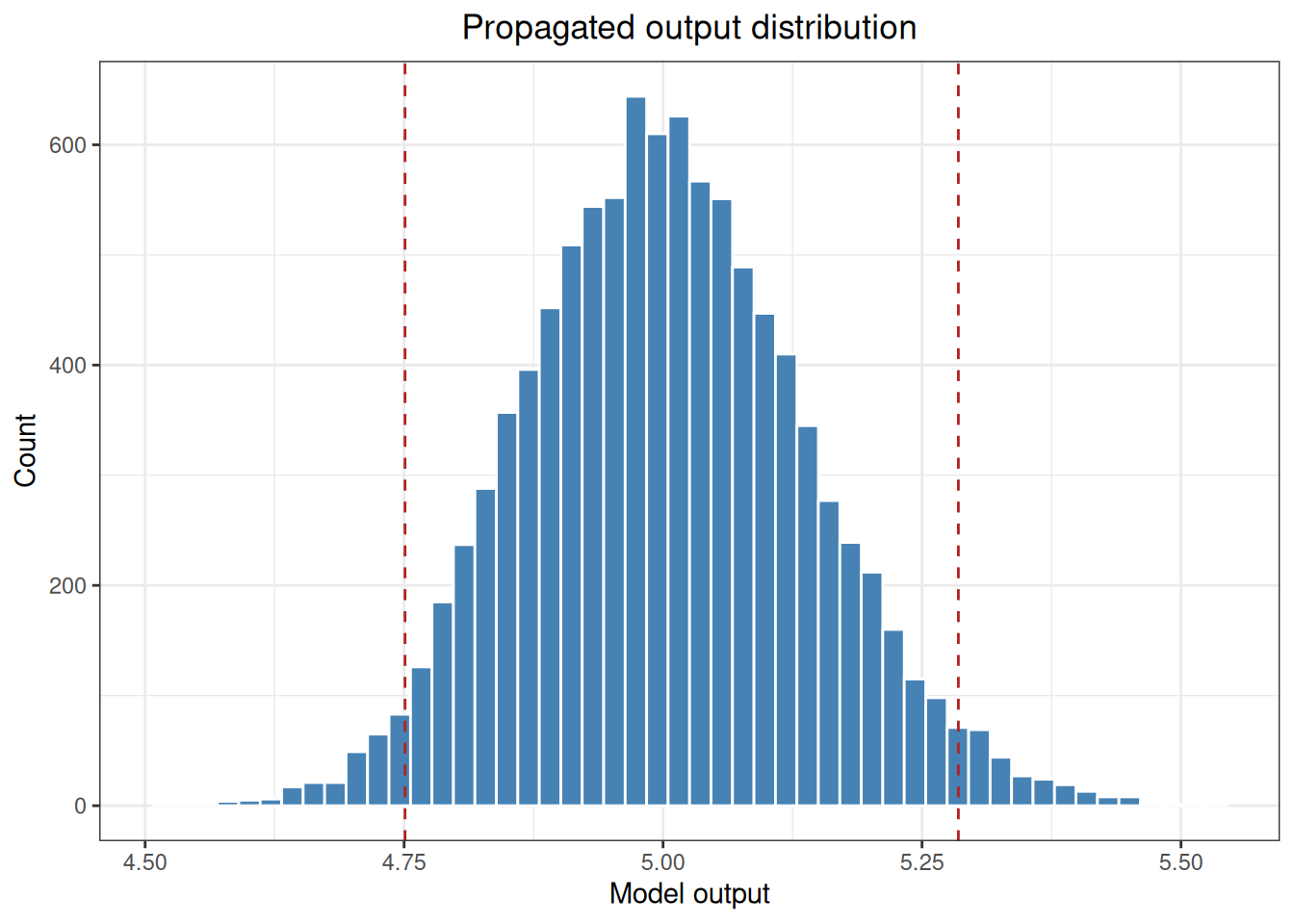
5.1.9 计量溯源链累计 uncertainty_traceability()
uncertainty_traceability() 按阶段记录新增分量,并返回每个阶段的累计预算。阶段名称应与质量体系中的校准链节点保持一致。
代码
trace <- uncertainty_traceability(
  stages = list(
    reference = list(certificate),
    assignment = list(repeatability),
    release = list(homogeneity_component$component)
  ),
  value = 100,
  coverage = 0.95,
  k = 2
)

trace
Traceability-chain uncertainty
  Stage: reference
    Introduced components           : 1
    Cumulative components           : 1
    Cumulative standard uncertainty : 1
    Relative standard uncertainty   : 0.01
    Coverage factor                 : 2
    Expanded uncertainty            : 2

  Stage: assignment
    Introduced components           : 1
    Cumulative components           : 2
    Cumulative standard uncertainty : 1.0076828
    Relative standard uncertainty   : 0.010076828
    Coverage factor                 : 2
    Expanded uncertainty            : 2.0153656

  Stage: release
    Introduced components           : 1
    Cumulative components           : 3
    Cumulative standard uncertainty : 1.5595164
    Relative standard uncertainty   : 0.015595164
    Coverage factor                 : 2
    Expanded uncertainty            : 3.1190328
uncertainty_traceability() 当前按阶段使用单位灵敏度和独立分量假设;如果某一阶段存在复杂测量模型或相关输入,应先用 uncertainty_propagate() 或 uncertainty_combine() 正确建模,再决定如何把节点结果传给后续阶段。
代码
plot(trace)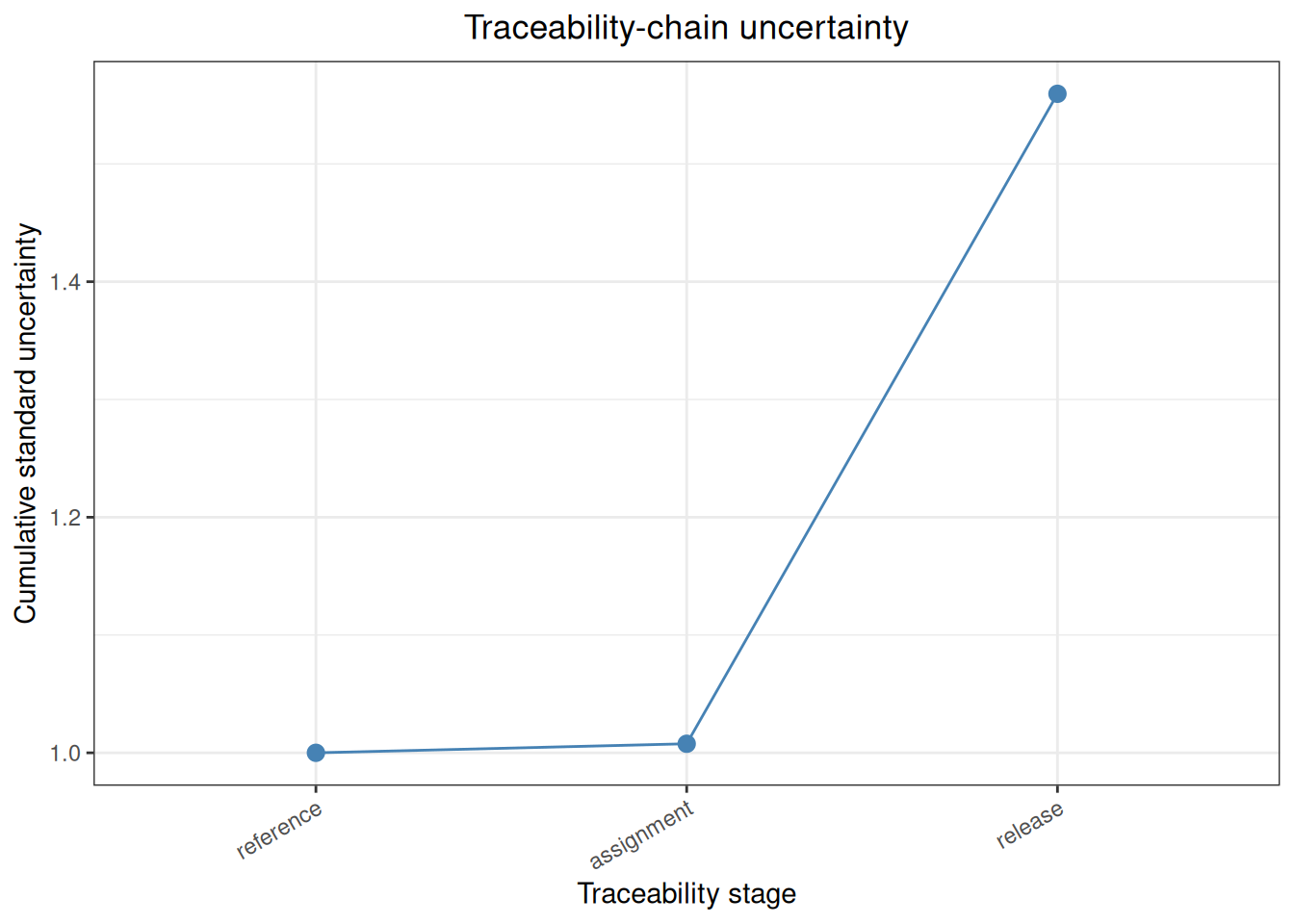
5.2 分析案例
5.2.1 CLSI EP29-A 附录 A:Type B 限值转换
CLSI EP29-A 附录 A 比较矩形、三角形和正态分布下,将 90~180 的限值区间转换为标准不确定度的结果,并给出称量规格、天平线性和重复性案例。以下使用 uncertainty_type_b() 和 uncertainty_combine() 重新计算;正态案例按标准原文的“±3 个标准差”解释,设置 coverage = 0.9973。
代码
ep29_a_rectangular <- uncertainty_type_b(
  "EP29 rectangular limits", estimate = 135,
  lower = 90, upper = 180, distribution = "rectangular"
)

ep29_a_triangular <- uncertainty_type_b(
  "EP29 triangular limits", estimate = 135,
  lower = 90, upper = 180, distribution = "triangular"
)

ep29_a_normal <- uncertainty_type_b(
  "EP29 normal limits", estimate = 135,
  lower = 90, upper = 180, distribution = "normal",
  coverage = 0.9973
)

ep29_a_weighing <- uncertainty_type_b(
  "EP29 weighing specification", estimate = 156,
  lower = 155, upper = 157, distribution = "rectangular"
)

ep29_a_linearity <- lapply(
  1:2,
  function(i) uncertainty_type_b(
    paste0("linearity ", i), estimate = 0,
    uncertainty = 0.02 / sqrt(6), distribution = "standard"
  )
)

ep29_a_repeatability <- lapply(
  1:2,
  function(i) uncertainty_type_b(
    paste0("repeatability ", i), estimate = 0,
    uncertainty = 0.01 / 3, distribution = "standard"
  )
)

ep29_a_balance <- uncertainty_combine(
  ep29_a_linearity[[1]], ep29_a_linearity[[2]],
  ep29_a_repeatability[[1]], ep29_a_repeatability[[2]],
  k = 1
)

ep29_a_tight <- uncertainty_combine(
  uncertainty_type_b(
    "EP29 tight specification", estimate = 156,
    lower = 155.9, upper = 156.1, distribution = "rectangular"
  ),
  uncertainty_type_b(
    "EP29 rounded balance", estimate = 0,
    uncertainty = 0.013, distribution = "standard"
  ),
  k = 1
)
从标准 PDF 附录 A 的原文结果检查表读取标准值,并逐项合并比较:
| appendix | statistic | standard | ivdtools |
|---|---|---|---|
| A | rectangular_90_180 | 26.000 | 25.9807621 |
| A | triangular_90_180 | 18.400 | 18.3711731 |
| A | gaussian_90_180 | 15.000 | 15.0001150 |
| A | weighing_specification_u | 0.577 | 0.5773503 |
| A | balance_u | 0.013 | 0.0124722 |
| A | tight_combined_u | 0.059 | 0.0591805 |
balance_u 使用未舍入的线性和重复性分量;紧限值案例按标准原文使用已舍入的 0.013 继续计算,因此末位差异来自中间舍入。
5.2.2 CLSI EP29-A 附录 B:胆固醇 IQC
附录 B 包含 42 个运行、每运行 3 次结果;标准将第 4 运行判定为技术可疑并排除,保留 41 个运行和 123 个结果。以下使用 uncertainty_iqc() 重新执行同一排除规则。
代码
ep29_b_data <- read_csv(
  "./data/005-不确定度分析/std-ep29-appendix-b.csv",
  show_col_types = FALSE
)
ep29_b_valid <- subset(ep29_b_data, run != 4L)
head(ep29_b_data, 6)
# A tibble: 6 × 5
run reagent_lot technician replicate cholesterol
<dbl> <chr> <chr> <dbl> <dbl>
1 1 A AK 1 7.9
2 1 A AK 2 7.9
3 1 A AK 3 8.1
4 2 A AK 1 7.5
5 2 A AK 2 7.3
6 2 A AK 3 7.6代码
ep29_b_iqc <- uncertainty_iqc(
  ep29_b_valid,
  result = "cholesterol",
  run = "run",
  quantity = "single",
  name = "EP29 cholesterol IQC"
)
提取 uncertainty_iqc() 返回的 ANOVA 统计量、综合标准不确定度和扩展不确定度,与 EP29-A 附录 B 的标准原文结果比较:
| appendix | statistic | standard | ivdtools |
|---|---|---|---|
| B | lot_A_rep1_mean | 7.60000 | 7.6500000 |
| B | lot_A_rep1_sd | 0.33000 | 0.2438723 |
| B | lot_B_rep1_mean | 7.71000 | 7.7142857 |
| B | lot_B_rep1_sd | 0.20000 | 0.2031889 |
| B | all_rep1_mean | 7.66000 | 7.6571429 |
| B | all_rep1_sd | 0.28000 | 0.2768665 |
| B | valid_rep1_mean | 7.68000 | 7.6829268 |
| B | valid_rep1_sd | 0.22000 | 0.2234977 |
| B | between_ss | 6.09000 | 6.0882927 |
| B | within_ss | 0.58000 | 0.5800000 |
| B | between_ms | 0.15200 | 0.1522073 |
| B | within_ms | 0.00707 | 0.0070732 |
| B | F | 21.50000 | 21.5189655 |
| B | p_value | 0.00000 | 0.0000000 |
| B | within_sd | 0.08400 | 0.0841021 |
| B | between_variance | 0.04830 | 0.0483780 |
| B | between_sd | 0.22000 | 0.2199501 |
| B | combined_u | 0.23500 | 0.2354808 |
| B | expanded_U | 0.47000 | 0.4709617 |
| B | grand_mean | 7.69000 | 7.6902439 |
| B | relative_expanded_percent | 6.10000 | 6.1241445 |
标准原文在批间方差和扩展不确定度计算中使用了已舍入的均方或分量,ivdtools 使用未舍入结果,因此个别末位存在中间量舍入差异。
5.2.3 CLSI EP29-A Example 1~3:测量模型传播
EP29-A Example 1~3 分别展示加减、乘法以及加乘除混合模型。它们适合用 uncertainty_combine() 和 uncertainty_propagate() 验证灵敏度系数、相关性和相对不确定度的处理。
代码
ep29_ex1_v1 <- uncertainty_type_b(
  "V1", estimate = 100, uncertainty = 0.1, distribution = "standard"
)

ep29_ex1_v2 <- uncertainty_type_b(
  "V2", estimate = 90, uncertainty = 0.2, distribution = "standard"
)

ep29_ex1_independent <- uncertainty_combine(
  ep29_ex1_v1, ep29_ex1_v2, value = 190, k = 1
)

ep29_ex1_equal <- uncertainty_combine(
  uncertainty_type_b("V1 equal", estimate = 100, uncertainty = 0.1,
                     distribution = "standard"),
  uncertainty_type_b("V2 equal", estimate = 100, uncertainty = 0.1,
                     distribution = "standard"),
  value = 200, k = 1
)

ep29_ex1_correlated <- uncertainty_combine(
  uncertainty_type_b("V1 same pipette", estimate = 100, uncertainty = 0.1,
                     distribution = "standard"),
  uncertainty_type_b("V2 same pipette", estimate = 100, uncertainty = 0.1,
                     distribution = "standard"),
  value = 200,
  correlation = matrix(c(1, 1, 1, 1), nrow = 2),
  k = 1
)

ep29_ex2 <- uncertainty_propagate(
  model = function(protein, volume) protein * volume,
  components = list(
    uncertainty_type_b("protein", estimate = 150, uncertainty = 3,
                       distribution = "standard"),
    uncertainty_type_b("volume", estimate = 1.5, uncertainty = 0.015,
                       distribution = "standard")
  )
)

ep29_ex3_staged <- uncertainty_propagate(
  model = function(numerator, denominator) numerator / denominator,
  components = list(
    uncertainty_type_b("numerator", estimate = 330, uncertainty = 11.1,
                       distribution = "standard"),
    uncertainty_type_b("denominator", estimate = 100, uncertainty = 3,
                       distribution = "standard")
  )
)

ep29_ex3_full <- uncertainty_propagate(
  model = function(c1, v1, c2, v2) (c1 * v1 + c2 * v2) / (v1 + v2),
  components = list(
    uncertainty_type_b("c1", estimate = 15, uncertainty = 0.2,
                       distribution = "standard"),
    uncertainty_type_b("v1", estimate = 10, uncertainty = 0.11,
                       distribution = "standard"),
    uncertainty_type_b("c2", estimate = 2, uncertainty = 0.1,
                       distribution = "standard"),
    uncertainty_type_b("v2", estimate = 90, uncertainty = 3,
                       distribution = "standard")
  )
)| appendix | statistic | standard | ivdtools |
|---|---|---|---|
| EP29 Example 1 | independent_unequal_u | 0.2200 | 0.2236068 |
| EP29 Example 1 | same_pipette_equal_u | 0.2000 | 0.2000000 |
| EP29 Example 1 | independent_equal_u | 0.1400 | 0.1414214 |
| EP29 Example 2 | relative_u | 0.0224 | 0.0223607 |
| EP29 Example 2 | absolute_u | 5.0300 | 5.0311529 |
| EP29 Example 3 | independent_staged_u | 0.1490 | 0.1487347 |
| EP29 Example 3 | correlated_u | 0.1000 | 0.1009289 |
Example 3 直接对原始混合模型传播时,重复出现在分子和分母中的体积量会自然产生协方差,因而得到约 0.10 mmol/L;标准原文把分子和分母先视为独立节点,给出约 0.149 mmol/L。两者采用的依赖结构不同,不能把这一差异归为显示舍入。
5.2.4 CLSI EP29-A Example 4:单因素 ANOVA 与 IQC 不确定度
Example 4 给出 5 个运行、每运行 5 次的血浆肌酐结果。它与 uncertainty_iqc() 的输入结构一致,适合检查批内、批间方差和单次结果综合不确定度。
代码
ep29_ex4_data <- data.frame(
  run = rep(1:5, each = 5),
  replicate = rep(1:5, times = 5),
  creatinine = c(
    140, 140, 140, 141, 140,
    138, 139, 138, 137, 139,
    143, 144, 144, 145, 143,
    143, 143, 142, 143, 142,
    142, 143, 141, 142, 143
  )
)

ep29_ex4_iqc <- uncertainty_iqc(
  ep29_ex4_data,
  result = "creatinine",
  run = "run",
  quantity = "single",
  name = "EP29 Example 4 P-Creatinine"
)| appendix | statistic | standard | ivdtools |
|---|---|---|---|
| EP29 Example 4 | ms_between | 24.40 | 24.4000000 |
| EP29 Example 4 | ms_within | 0.52 | 0.5200000 |
| EP29 Example 4 | within_sd | 0.72 | 0.7211103 |
| EP29 Example 4 | between_sd | 2.19 | 2.1854061 |
| EP29 Example 4 | combined_u | 2.30 | 2.3013040 |
| EP29 Example 4 | F | 46.90 | 46.9230769 |
F 值的末位差异来自标准原文的显示舍入,函数使用未舍入均方计算。
5.2.5 CLSI EP29-A Example 5~6:偏倚估计及偏倚校正不确定度
Example 5 只有汇总统计量,没有原始差值数据,因此用 uncertainty_type_b() 保存标准原文给出的汇总标准不确定度,再用 uncertainty_combine() 合成。Example 6a 使用有证参考物质的赋值不确定度和实验室均值不确定度。
代码
ep29_ex5_make <- function(n) {
  uncertainty_combine(
    uncertainty_type_b(
      "test method imprecision", estimate = 0,
      uncertainty = 0.71, distribution = "standard"
    ),
    uncertainty_type_b(
      paste0("bias estimate n=", n), estimate = 0,
      uncertainty = 1.2 / sqrt(n), distribution = "standard"
    ),
    k = 1
  )
}
ep29_ex5_n144 <- ep29_ex5_make(144)
ep29_ex5_n16 <- ep29_ex5_make(16)

ep29_ex6a_lab_mean <- uncertainty_type_b(
  "CRM laboratory mean", estimate = 6.04,
  uncertainty = 0.045, distribution = "standard"
)
ep29_ex6a_crm <- uncertainty_type_b(
  "CRM certified value", estimate = 6.3,
  uncertainty = 0.1, k = 2, distribution = "standard"
)
ep29_ex6a_bias <- uncertainty_combine(
  ep29_ex6a_lab_mean, ep29_ex6a_crm, value = 6.04 - 6.3, k = 1
)

ep29_ex6b_claim <- uncertainty_combine(
  uncertainty_type_b(
    "future result, literature claim", estimate = 6.04,
    uncertainty = 0.035 * 6.04, distribution = "standard"
  ),
  uncertainty_type_b(
    "bias correction", estimate = 0, uncertainty = 0.068,
    distribution = "standard"
  ),
  k = 1
)
ep29_ex6b_lab <- uncertainty_combine(
  uncertainty_type_b(
    "future result, local ANOVA", estimate = 6.04,
    uncertainty = 0.151, distribution = "standard"
  ),
  uncertainty_type_b(
    "bias correction", estimate = 0, uncertainty = 0.068,
    distribution = "standard"
  ),
  k = 1
)| appendix | statistic | standard | ivdtools |
|---|---|---|---|
| EP29 Example 5 | n144_bias_u | 0.100 | 0.1000000 |
| EP29 Example 5 | n144_combined_u | 0.720 | 0.7170077 |
| EP29 Example 5 | n16_bias_u | 0.300 | 0.3000000 |
| EP29 Example 5 | n16_combined_u | 0.770 | 0.7707788 |
| EP29 Example 6a | measured_mean | 6.040 | 6.0400000 |
| EP29 Example 6a | bias | -0.260 | -0.2600000 |
| EP29 Example 6a | bias_u | 0.068 | 0.0672681 |
| EP29 Example 6a | bias_expanded | 0.140 | 0.1345362 |
| EP29 Example 6b | claim_combined_u | 0.220 | 0.2220675 |
| EP29 Example 6b | lab_combined_u | 0.165 | 0.1656050 |
Example 6a 的偏倚及其不确定度同时纳入实验室均值和有证参考物质赋值的不确定度;Example 6b 分别采用文献精密度和本实验室精密度,因此两个情景不可互换。
5.2.6 CLSI EP29-A Example 10:肌酐清除率不确定度传播
EP29-A Example 10 给出肌酐清除率的测量模型,并分别提供尿肌酐、血清肌酐、尿液体积、收集时间和前分析体积的不确定度。以下将原文输入量建立为 B 类组件,并用 uncertainty_propagate(method = “delta”) 传播:
代码
ep29_u_crea <- uncertainty_type_b(
  "u_crea", estimate = 15, uncertainty = 0.45,
  distribution = "standard"
)
ep29_u_vol <- uncertainty_type_b(
  "u_vol", estimate = 1500, uncertainty = 22.5,
  distribution = "standard"
)
ep29_s_crea <- uncertainty_type_b(
  "s_crea", estimate = 0.115, uncertainty = 0.00575,
  distribution = "standard"
)
ep29_time <- uncertainty_type_b(
  "time", estimate = 1440, uncertainty = 15,
  distribution = "standard"
)
ep29_u_vol_prea <- uncertainty_type_b(
  "u_vol_prea", estimate = 100,
  lower = 0, upper = 200,
  distribution = "rectangular"
)

ep29_creatinine_clearance <- uncertainty_propagate(
  model = function(u_crea, u_vol, s_crea, time, u_vol_prea) {
    (u_vol + u_vol_prea) * u_crea / (s_crea * time)
  },
  components = list(
    ep29_u_crea, ep29_u_vol, ep29_s_crea,
    ep29_time, ep29_u_vol_prea
  ),
  method = "delta"
)| appendix | statistic | standard | ivdtools |
|---|---|---|---|
| EP29 Example 10 | estimate | 145.0 | 144.927536 |
| EP29 Example 10 | relative_percent | 7.1 | 7.076966 |
EP29-A Figure 4 的 Kragten 数值近似给出约 6.9% 的相对合成不确定度,而 uncertainty_propagate() 的一阶 delta 结果约为 7.1%。这一差异来自数值近似路径,不是输入数据差异。
5.2.7 CLSI EP29-A Example 11:线性回归预测方程
Example 11 用 A1C 预测 eAG,测量模型为 \(eAG = \alpha + \beta A1C + \epsilon\)。以下使用 uncertainty_propagate() 传播截距、斜率、A1C 测量值和预测误差的不确定度,并按标准 Table 4 的参数在 A1C = 7% 处计算三个情景。
代码
ep29_ex11_make <- function(relative_a1c_u) {
  a1c <- 7
  uncertainty_propagate(
    model = function(alpha, beta, A1C, epsilon) {
      alpha + beta * A1C + epsilon
    },
    components = list(
      uncertainty_type_b("alpha", estimate = -46.6, uncertainty = 3.8,
                         distribution = "standard"),
      uncertainty_type_b("beta", estimate = 28.7, uncertainty = 0.6,
                         distribution = "standard"),
      uncertainty_type_b("A1C", estimate = a1c,
                         uncertainty = relative_a1c_u * a1c,
                         distribution = "standard"),
      uncertainty_type_b("epsilon", estimate = 0,
                         uncertainty = 2.21 * a1c,
                         distribution = "standard")
    )
  )
}
ep29_ex11_results <- lapply(c(0, 0.02, 0.05), ep29_ex11_make)| appendix | statistic | standard | ivdtools |
|---|---|---|---|
| EP29 Example 11 | A1C_7_U_0pct | 30.8 | 32.94850 |
| EP29 Example 11 | A1C_7_U_2pct | 31.8 | 33.91432 |
| EP29 Example 11 | A1C_7_U_5pct | 36.8 | 38.59031 |
标准 Table 4 的截距—斜率协方差项因原文参数已舍入,直接构造的相关矩阵不满足正半定条件;因此表中 ivdtools 列采用独立输入的 delta 传播,standard 列采用标准 Equation 32 的协方差公式重算结果,差异来自相关项处理方式。
5.2.8 YY/T 1709:校准物均匀性、稳定性和定值不确定度
5.2.8.1 附录 A:均匀性引入的不确定度
代码
yyt1709_homogeneity_data <- read_csv(
  "./data/005-不确定度分析/std-yyt1709-homogeneity.csv",
  show_col_types = FALSE
)
yyt1709_homogeneity <- uncertainty_homogeneity(
  yyt1709_homogeneity_data,
  unit = "bottle",
  result = "result",
  name = "YY/T 1709 瓶间均匀性"
)
5.2.8.2 附录 B:稳定性引入的不确定度
标准原文按各时间点的均值进行线性趋势计算。为保持与标准相同的统计口径,先按时间点汇总,再将汇总结果传给 uncertainty_stability();如果把所有瓶内重复直接作为独立回归行,斜率标准误会采用不同的信息量。
代码
yyt1709_stability_data <- read_csv(
  "./data/005-不确定度分析/std-yyt1709-stability.csv",
  show_col_types = FALSE
)

yyt1709_timepoint_means <- function(data) {
  aggregate(result ~ time, data = data, FUN = mean)
}

yyt1709_stability_results <- list(
  长期 = uncertainty_stability(
    yyt1709_timepoint_means(subset(yyt1709_stability_data, study == "长期")),
    time = "time", result = "result", shelf_life = 18,
    name = "长期稳定性"
  ),
  运输室温 = uncertainty_stability(
    yyt1709_timepoint_means(subset(yyt1709_stability_data, study == "运输室温")),
    time = "time", result = "result", shelf_life = 7,
    name = "运输稳定性(室温)"
  ),
  运输37C = uncertainty_stability(
    yyt1709_timepoint_means(subset(yyt1709_stability_data, study == "运输37C")),
    time = "time", result = "result", shelf_life = 7,
    name = "运输稳定性(37 C)"
  ),
  复溶 = uncertainty_stability(
    yyt1709_timepoint_means(subset(yyt1709_stability_data, study == "复溶")),
    time = "time", result = "result", shelf_life = 7,
    name = "复溶稳定性"
  )
)
5.2.8.3 附录 C:定值不确定度合成
工作校准品证书和复溶信息先转换为 B 类组件,赋值重复性由 uncertainty_type_a() 估计,最终使用 uncertainty_combine() 合成相对和绝对不确定度。
代码
yyt1709_assignment <- read_csv(
  "./data/005-不确定度分析/std-yyt1709-assignment.csv",
  show_col_types = FALSE
)

yyt1709_assignment_u <- uncertainty_type_a(
  yyt1709_assignment$result,
  name = "赋值重复性",
  quantity = "mean",
  relative = TRUE
)

yyt1709_assigned_mean <- mean(yyt1709_assignment$result)

yyt1709_working_calibration <- uncertainty_type_b(
  "工作校准品",
  estimate = 178.06,
  uncertainty = 6.01,
  distribution = "standard",
  k = 2,
  relative = TRUE
)
yyt1709_reconstitution_1 <- uncertainty_type_b(
  "工作校准品复溶",
  estimate = 1,
  uncertainty = 0.00003 / (sqrt(3) * 0.99758),
  distribution = "standard",
  k = 1,
  relative = TRUE
)
yyt1709_reconstitution_2 <- uncertainty_type_b(
  "产品校准品复溶",
  estimate = 1,
  uncertainty = 0.01 / sqrt(3),
  distribution = "standard",
  k = 1,
  relative = TRUE
)

yyt1709_reconstitution <- uncertainty_combine(
  yyt1709_reconstitution_1,
  yyt1709_reconstitution_2,
  k = 1
)
yyt1709_characterization_budget <- uncertainty_combine(
  yyt1709_working_calibration,
  yyt1709_assignment_u,
  yyt1709_reconstitution_1,
  yyt1709_reconstitution_2,
  value = yyt1709_assigned_mean,
  coverage = 0.95,
  k = 2
)
这里传入的 uncertainty 已是标准不确定度,因此使用 distribution = "standard" 表示函数不再进行分布换算。两个式子中的 sqrt(3) 用于将矩形分布的允许半宽换算为标准不确定度;第一项中的 0.99758 是实际称量质量,用于把绝对称量误差转换为相对误差,不是分布参数。
5.2.8.4 附录 A~C:与 YY/T 1709 原文结果对照
| appendix | statistic | standard | ivdtools |
|---|---|---|---|
| A(均匀性) | SS_between | 0.2114405 | 0.2114405 |
| A(均匀性) | SS_within | 0.3556000 | 0.3556000 |
| A(均匀性) | MS_between | 0.0162647 | 0.0162647 |
| A(均匀性) | MS_within | 0.0127000 | 0.0127000 |
| A(均匀性) | F | 1.2806810 | 1.2806813 |
| A(均匀性) | u_bb | 0.0344916 | 0.0344705 |
| C(定值) | mean | 179.7300000 | 179.7294000 |
| C(定值) | u_REP_rel | 0.0012560 | 0.0012556 |
| C(定值) | u_wcal_rel | 0.0168763 | 0.0168763 |
| C(定值) | u_sol_rel | 0.0057735 | 0.0057735 |
| C(定值) | u_char_rel | 0.0178900 | 0.0178807 |
| C(定值) | u_char | 3.2200000 | 3.2136942 |
| C(赋值确认) | mean | 107.7200000 | 107.7240000 |
| C(赋值确认) | bias | -0.3800000 | -0.3760000 |
| B(长期) | slope | -0.0137000 | -0.0137302 |
| B(长期) | intercept | 50.0114000 | 50.0114286 |
| B(长期) | residual_sd | 0.3238000 | 0.3237945 |
| B(长期) | slope_se | 0.0204000 | 0.0203971 |
| B(长期) | u_stability | 0.3672000 | 0.3671484 |
| B(运输室温) | slope | -0.0487000 | -0.0486706 |
| B(运输室温) | intercept | 50.3568000 | 50.3568056 |
| B(运输室温) | residual_sd | 0.5451000 | 0.5297030 |
| B(运输室温) | slope_se | 0.0841000 | 0.0817349 |
| B(运输室温) | u_stability | 0.5887000 | 0.5721446 |
| B(运输37C) | slope | -0.0330000 | -0.0329960 |
| B(运输37C) | intercept | 50.3936000 | 50.3936111 |
| B(运输37C) | residual_sd | 0.4310000 | 0.4220273 |
| B(运输37C) | slope_se | 0.0665000 | 0.0651202 |
| B(运输37C) | u_stability | 0.4655000 | 0.4558416 |
| B(复溶) | slope | 0.0433000 | 0.0432540 |
| B(复溶) | intercept | 49.6536000 | 49.6536111 |
| B(复溶) | residual_sd | 0.6319000 | 0.6214551 |
| B(复溶) | slope_se | 0.0975000 | 0.0958926 |
| B(复溶) | u_stability | 0.6825000 | 0.6712482 |