16 检出限/定量限

本文围绕空白限（LoB）、检出限（LoD）、定量限（LoQ）及其声明验证，说明如何把低浓度实验数据转换为可审计的灵敏度结论。不同指标回答的问题不同：LoB 描述空白分布上界，LoD 描述检出能力，LoQ 还必须附带精密度或总误差要求。

分析流程：建立或验证 LoB、LoD、LoQ

%%{init: {"theme":"base","themeVariables":{"primaryColor":"#EAF2FB","primaryBorderColor":"#2780E3","primaryTextColor":"#212529","lineColor":"#6C757D","secondaryColor":"#EAF7E6","tertiaryColor":"#FFF4E8","fontSize":"13px"},"flowchart":{"nodeSpacing":18,"rankSpacing":24,"padding":6}}}%%

flowchart LR
    A["明确 LoB、LoD、LoQ<br/>或声明验证目标"] --> B["sensitivity_design()<br/>核对设计"]
    B --> C["sensitivity_lob()"]
    C --> D["sensitivity_lod()"]
    D --> E["sensitivity_loq()"]
    E --> F["sensitivity_verify()"]
    F --> G["检查方法、精密度轮廓<br/>和验证通过率"]

    classDef input fill:#EAF2FB,stroke:#2780E3,color:#212529
    classDef process fill:#EAF7E6,stroke:#3FB618,color:#212529
    classDef output fill:#F4EEFB,stroke:#9954BB,color:#212529
    class A input
    class B,C,D,E,F process
    class G output

代码

library(ivdtools)

16.1 主要函数

分析灵敏度模块使用原始长数据作为主要输入，并将限值建立、声明验证和试验设计分开：

函数	用途
`sensitivity_lob()`	非参数、参数或零 LoB 建立
`sensitivity_lod()`	经典、非参数试验、精密度曲线或 Probit LoD
`sensitivity_loq()`	Westgard、RMS、精密度或自定义目标 LoQ
`sensitivity_verify()`	验证已有 LoB、LoD 或 LoQ 声明
`sensitivity_design()`	查看最低设计要求和实际数据计数

16.1.1 建立函数、参数与核心统计量

代码

sensitivity_lob(
  data, result, sample, lot = NULL,
  method = c("nonparametric", "parametric", "zero"),
  alpha = 0.05, lot_rule = c("ep17", "separate", "combined"),
  exclude = NULL
)
sensitivity_lod(
  data, result = NULL, sample = NULL, lob, lot = NULL,
  concentration = NULL, detected = NULL,
  method = c("classical", "nonparametric", "profile", "probit"),
  beta = 0.05, profile_model = c("linear", "quadratic", "sadler", "vfp")
)
sensitivity_loq(
  data, result, sample, assigned, lot = NULL,
  method = c("westgard", "rms", "precision", "custom"),
  goal, goal_scale = c("relative", "absolute"),
  lod = NULL, k = 2, profile = FALSE
)

非参数 LoB 是空白结果的 \(1-\alpha\) 秩分位数；参数法使用

\[ LoB=\bar x_B+c_p s_B, \]

其中 \(c_p\) 根据 \(\alpha\) 和空白自由度 \(B-K\) 作有限样本修正。method="zero" 固定 \(LoB=0\)，并报告空白大于零的比例。经典 LoD 对多个低水平样本先按自由度合并 SD：

\[ s_p=\sqrt{\frac{\sum_j(n_j-1)s_j^2}{\sum_j(n_j-1)}}, \]

再结合 LoB、\(\beta\) 和有限样本修正得到检出限。精密度轮廓法求解浓度相关 SD，Probit 法则拟合检测概率—浓度关系；两者的数据结构和假设不同。

LoQ 的逐水平偏差 \(b=\bar x-x_a\)。四种误差量为：

`method`	与 `goal` 比较的原始量
`westgard`	\(\|b\|+k s\)
`rms`	\(\sqrt{s^2+b^2}\)
`precision`	\(s\)
`custom`	`accuracy_function()` 返回值

goal_scale="relative" 时再除以 \(|x_a|\)。候选 LoQ 是满足目标的最低观测均值或拟合轮廓交点；多批按所选 lot_rule 处理，最终取最保守的有限候选值。提供 LoD 时 \(LoQ_{\mathrm{reported}}=\max(LoQ_{\mathrm{candidate}},LoD)\)。

sensitivity_lob()、sensitivity_lod() 和 sensitivity_loq() 返回对应限值、方法、核心统计量和诊断信息。

16.1.2 声明验证和设计检查

代码

sensitivity_verify(
  data, result, sample, limit = c("lob", "lod", "loq"),
  claim, lob = NULL, assigned = NULL, allowable_error = NULL,
  error_scale = c("relative", "absolute"), alpha = 0.05
)
sensitivity_design(method = "all", data = NULL, ...)

LoB 验证统计 \(x\le claim\)，LoD 验证统计 \(x\ge LoB\)，LoQ 验证统计结果是否在赋值允许误差窗内。函数输出观察成功比例、单侧 Wilson score 区间以及 EP17 表 1 边界，但故意不生成 pass 字段。 sensitivity_design() 给出最低设计要求并可汇总实际数据计数；它只显示差距，不替代方案判定。

sensitivity_verify() 返回观察成功比例、Wilson 区间和边界信息；sensitivity_design() 返回最低要求与实际计数表。

16.2 分析案例

16.2.1 LoB

原始数据每行是一条测量结果：

代码

# 模拟数据
set.seed(17)
blank <- expand.grid(
  lot = c("A", "B"), sample = paste0("blank", 1:4), replicate = 1:15
)
blank$result <- rnorm(nrow(blank), 0.2, 0.1)
head(blank, 6)

  lot sample replicate     result
1   A blank1         1 0.09849913
2   B blank1         1 0.19203633
3   A blank2         1 0.17670130
4   B blank2         1 0.11827321
5   A blank3         1 0.27720908
6   B blank3         1 0.18343881

代码

# lob 建立
lob_np <- sensitivity_lob(
  blank, result = "result", sample = "sample", lot = "lot",
  method = "nonparametric"
)
lob_np

Analytical sensitivity: LOB 
  Method: nonparametric 
  Estimate: 0.378828

EP17 批号规则默认用于全部建立函数：2～3 批分别计算并取最大值，4 批及以上合并计算。负测量结果不会被自动截断为 0。

16.2.2 LoD

经典 LoD 使用低水平样本的合并 SD：

代码

# 模拟数据
low <- expand.grid(
  lot = c("A", "B"), sample = paste0("low", 1:4), replicate = 1:15
)
low$result <- rnorm(nrow(low), 1.2, 0.2)
head(low, 6)

  lot sample replicate    result
1   A   low1         1 1.4763513
2   B   low1         1 1.2897865
3   A   low2         1 1.1695380
4   B   low2         1 1.2518588
5   A   low3         1 0.8777197
6   B   low3         1 0.7982088

代码

# lod 建立
lod_classical <- sensitivity_lod(
  low, result = "result", sample = "sample", lot = "lot",
  lob = lob_np, method = "classical"
)
lod_classical

Analytical sensitivity: LOD 
  Method: classical 
  Estimate: 0.771614

method = "profile" 支持 linear、quadratic、sadler 和 vfp 精度轮廓；method = "probit" 支持原始 0/1 检测结果或命中数/总数汇总数据。Cochran 统计量和拟合指标只作为诊断信息，不由程序代替用户选择分析路径。

16.2.3 LoQ

LoQ 的准确度目标必须预先给定。相对目标使用比例，例如 21.6% 写作 0.216：

代码

# 模拟数据
loq_data <- expand.grid(
  lot = c("A", "B"), sample = paste0("pool", 1:4), replicate = 1:9
)
loq_data$assigned <- rep(rep(c(30, 35, 40, 45), each = 9), 2)
loq_data$result <- rnorm(nrow(loq_data), loq_data$assigned,
                         0.06 * loq_data$assigned)
head(loq_data, 6)

  lot sample replicate assigned   result
1   A  pool1         1       30 29.70842
2   B  pool1         1       30 28.62287
3   A  pool2         1       30 29.82049
4   B  pool2         1       30 30.07043
5   A  pool3         1       30 28.84843
6   B  pool3         1       30 28.98056

代码

# loq 建立
loq_te <- sensitivity_loq(
  loq_data, result = "result", sample = "sample", assigned = "assigned",
  lot = "lot", method = "westgard", goal = 0.216,
  goal_scale = "relative", lod = lod_classical
)
loq_te

Analytical sensitivity: LOQ 
  Method: westgard 
  Estimate: 29.4924 
  Candidate LoQ: 29.4924 
  Reported LoQ : 29.4924

结果同时保存 candidate_loq 与 reported_loq，因此 LoD 约束不会覆盖原始候选值。

16.2.4 声明验证

limit 每次只能指定一种声明：

代码

# 模拟数据
verification <- data.frame(
  sample = rep(c("blank1", "blank2"), each = 10),
  result = c(rep(0, 19), 1.2)
)
head(verification, 6)

  sample result
1 blank1      0
2 blank1      0
3 blank1      0
4 blank1      0
5 blank1      0
6 blank1      0

代码

# lob 验证
v_lob <- sensitivity_verify(
  verification, result = "result", sample = "sample",
  limit = "lob", claim = 1
)
v_lob

Analytical sensitivity: VERIFICATION 
  Method: lob 
  Limit                    : lob
  Claim                    : 1
  LoB                      : 1
  Total results            : 20
  Consistent results       : 19
  Observed proportion      : 0.95
  Score CI lower           : 0.80399276
  Score CI upper           : 0.98876518
  EP17 boundary            : 0.85
  Difference from boundary : 0.1

LoB：统计 result <= claim。
LoD：统计 result >= lob；LoD 声明值不是检测判定阈值。
LoQ：统计结果是否落入各样本赋值的允许误差窗口。

结果包含观察比例、单侧 Wilson score 区间、EP17 Table 1 边界及差值，不包含 pass 或 verified 字段。

16.2.5 试验设计

代码

sensitivity_design("all")

Analytical sensitivity study design
  Method: classical
    Reagent lots         : 2
    Instruments          : 1
    Days                 : 3
    Blank samples        : 4
    Low samples          : 4
    Concentration levels : NA
    Replicates per lot   : 60
    Replicate scope      : blank and low results separately

  Method: profile
    Reagent lots         : 2
    Instruments          : 1
    Days                 : 5
    Blank samples        : 0
    Low samples          : 5
    Concentration levels : 5
    Replicates per lot   : 40
    Replicate scope      : per sample

  Method: probit
    Reagent lots         : 2
    Instruments          : NA
    Days                 : NA
    Blank samples        : 0
    Low samples          : 3
    Concentration levels : 5
    Replicates per lot   : 20
    Replicate scope      : per sample and concentration level

  Method: loq
    Reagent lots         : 2
    Instruments          : 1
    Days                 : 3
    Blank samples        : 0
    Low samples          : 4
    Concentration levels : 1
    Replicates per lot   : 36
    Replicate scope      : total low results

  Method: verification
    Reagent lots         : 1
    Instruments          : 1
    Days                 : 3
    Blank samples        : 2
    Low samples          : 0
    Concentration levels : 1
    Replicates per lot   : 20
    Replicate scope      : total verification results

代码

sensitivity_design("verification", verification,
                   result = "result", sample = "sample", limit = "lob")

Analytical sensitivity study design
  Method               : verification
  Reagent lots         : 1
  Instruments          : 1
  Days                 : 3
  Blank samples        : 2
  Low samples          : 0
  Concentration levels : 1
  Replicates per lot   : 20
  Replicate scope      : total verification results

Observed study counts
  Observations         : 20
  Reagent lots         : NA
  Days                 : NA
  Samples              : 2
  Concentration levels : NA

设计对象并列报告最低要求与实际计数，但不作通过或不通过结论。排除记录必须通过 exclude 显式传入，并会保存在结果对象中。

16.2.6 标准案例：CLSI EP17-A2 附录 A：经典法 LoB 和 LoD

两批试剂各有 60 个空白和 60 个低水平结果。按 EP17 的批号规则分别计算后取较大值。

代码

ep17_blank <- read.csv("./data/016-分析灵敏度/std-ep17-appendix-a-blank.csv", check.names = FALSE)
ep17_low <- read.csv("./data/016-分析灵敏度/std-ep17-appendix-a-low.csv", check.names = FALSE)

ep17_lob_np <- sensitivity_lob(
  ep17_blank, result = "result", sample = "sample", lot = "lot",
  method = "nonparametric"
)
ep17_lod_np <- sensitivity_lod(
  ep17_low, result = "result", sample = "sample", lot = "lot",
  lob = ep17_lob_np, method = "classical"
)
ep17_lob_p <- sensitivity_lob(
  ep17_blank, result = "result", sample = "sample", lot = "lot",
  method = "parametric"
)
ep17_lod_p <- sensitivity_lod(
  ep17_low, result = "result", sample = "sample", lot = "lot",
  lob = ep17_lob_p, method = "classical"
)

EP17-A2 附录 A：ivdtools 与标准原文结果对照
标准位置	统计量	标准结果	ivdtools结果
EP17-A2 Appendices A	nonparametric LoB lot 1	7.6	7.6000
EP17-A2 Appendices A	nonparametric LoB lot 2	9.4	9.4000
EP17-A2 Appendices A	nonparametric LoB report	9.4	9.4000
EP17-A2 Appendices A	classical LoD lot 1	14.5	14.5309
EP17-A2 Appendices A	classical LoD lot 2	13.8	13.8343
EP17-A2 Appendices A	classical LoD report	14.5	14.5309
EP17-A2 Appendices A	parametric LoB report	8.8	8.7956
EP17-A2 Appendices A	parametric LoD report	13.9	13.9266

负测量结果按原表保留，未截断为 0。

16.2.7 标准案例：CLSI EP17-A2 附录 C：Probit LoD

零浓度的三批 66 次结果全部阴性，支持本案例 LoB = 0。对数浓度拟合时零浓度不能取对数，因此只将阳性浓度行送入 Probit 模型；零浓度计数仍保留在输入表中供 LoB 核对。

代码

ep17_probit <- read.csv("./data/016-分析灵敏度/std-ep17-appendix-c-probit.csv", check.names = FALSE)
ep17_probit_fit_data <- ep17_probit[ep17_probit$concentration > 0, ]

ep17_c_lod <- sensitivity_lod(
  ep17_probit_fit_data,
  result = "positive", sample = "sample", lob = 0, lot = "lot",
  concentration = "concentration", detected = "positive", total = "total",
  method = "probit", concentration_scale = "log10"
)
plot(ep17_c_lod)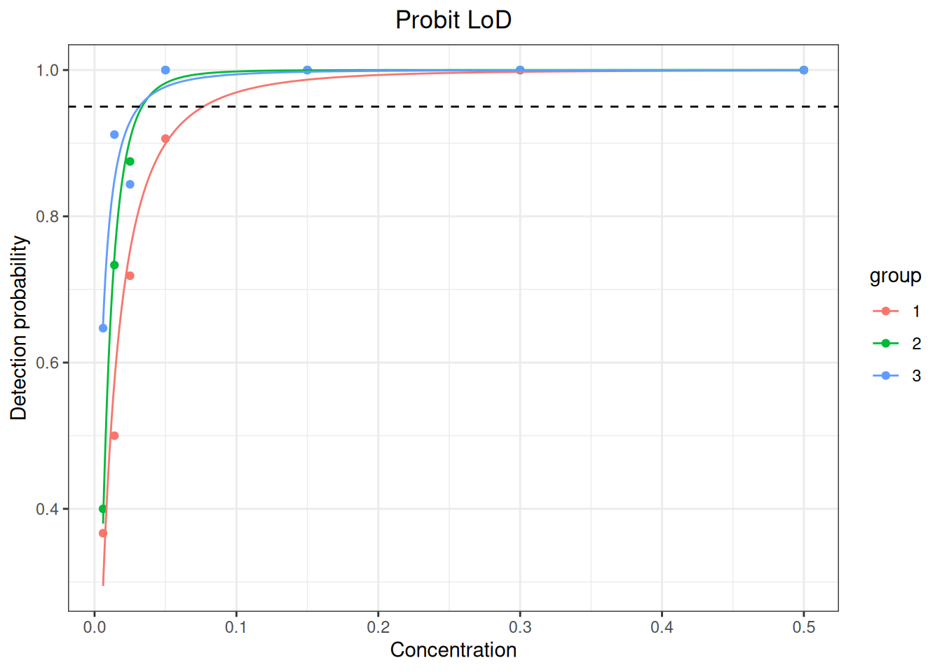

EP17-A2 附录 C：ivdtools 与标准原文结果对照
标准位置	统计量	标准结果	ivdtools结果
EP17-A2 Appendix C	Probit LoD lot 1	0.077	0.0766
EP17-A2 Appendix C	Probit LoD lot 2	0.033	0.0335
EP17-A2 Appendix C	Probit LoD lot 3	0.031	0.0314

三批 LoD 分别为 0.077、0.033 和 0.031 CFU/mL；取最大值得报告 LoD 0.077 CFU/mL。两类拟合优度检验均未提示失拟，但本附录仅使用 1 个样品，是标准为简化示例而明确偏离最低 3 个样品要求的设计，不能当作合规研究模板。

16.2.8 标准案例：CLSI EP17-A2 附录 E、F：声明验证

代码

ep17_ef <- read.csv("./data/016-分析灵敏度/std-ep17-appendix-e-verification.csv", check.names = FALSE)
ep17_f <- read.csv("./data/016-分析灵敏度/std-ep17-appendix-f-loq-verification.csv", check.names = FALSE)

ep17_verify_lob <- sensitivity_verify(
  ep17_ef[ep17_ef$type == "blank", ],
  result = "result", sample = "sample", limit = "lob", claim = 20
)
ep17_verify_lod <- sensitivity_verify(
  ep17_ef[ep17_ef$type == "positive", ],
  result = "result", sample = "sample", limit = "lod", claim = 45,
  lob = 20
)
ep17_verify_loq <- sensitivity_verify(
  ep17_f, result = "result", sample = "sample", limit = "loq", claim = 50,
  assigned = "target", allowable_error = 0.15
)

EP17-A2 附录 E～F：ivdtools 与标准原文结果对照
标准位置	统计量	标准结果	ivdtools结果
EP17-A2 Appendices E-F	LoB consistency (%)	95.8	95.8333
EP17-A2 Appendices E-F	LoD consistency (%)	91.7	91.6667
EP17-A2 Appendices E-F	LoQ consistency (%)	91.1	91.1111

16.2.9 标准案例：YY/T 1789.3—2022 附录 A ProGRP

附录 A 给出两批试剂各 60 个空白结果和 60 个低浓度结果，适合直接使用 sensitivity_lob() 与 sensitivity_lod()。原表中的负空白值原样保留，不截断为零。

代码

yyt1789_3_blank <- read.csv(
  "./data/016-分析灵敏度/std-yyt1789-3-appendix-a-blank.csv"
)
yyt1789_3_low <- read.csv(
  "./data/016-分析灵敏度/std-yyt1789-3-appendix-a-low.csv"
)

yyt1789_3_lob_np <- sensitivity_lob(
  yyt1789_3_blank, result = "result", sample = "sample", lot = "lot",
  method = "nonparametric"
)
yyt1789_3_lob_p <- sensitivity_lob(
  yyt1789_3_blank, result = "result", sample = "sample", lot = "lot",
  method = "parametric"
)
yyt1789_3_lod_classical <- sensitivity_lod(
  yyt1789_3_low, result = "result", sample = "sample", lot = "lot",
  lob = yyt1789_3_lob_np, method = "classical"
)
yyt1789_3_lod_np <- sensitivity_lod(
  yyt1789_3_low, result = "result", sample = "sample", lot = "lot",
  lob = yyt1789_3_lob_np, method = "nonparametric"
)

YY/T 1789.3—2022 附录 A：ivdtools 与标准结果对照
标准位置	统计量	标准结果	ivdtools结果
YY/T 1789.3 Appendix A	nonparametric LoB lot 1	0.240	0.2450
YY/T 1789.3 Appendix A	nonparametric LoB lot 2	0.250	0.2500
YY/T 1789.3 Appendix A	reported LoB	0.250	0.2500
YY/T 1789.3 Appendix A	parametric LoB lot 1	0.174	0.1758
YY/T 1789.3 Appendix A	parametric LoB lot 2	0.176	0.1779
YY/T 1789.3 Appendix A	classical LoD lot 1	0.350	0.3570
YY/T 1789.3 Appendix A	classical LoD lot 2	0.360	0.3673
YY/T 1789.3 Appendix A	nonparametric LoD lot 1	1.075	1.0750
YY/T 1789.3 Appendix A	nonparametric LoD lot 2	1.130	1.1300

中间量存在3处必须披露的算法差异：

标准的非参数 LoB 直接取第 57 位，包使用连续秩 57.5 并在第 57、58 位之间插值，所以批 1 为 0.245 而不是 0.24；两批取较大值后报告值恰好仍为 0.25。
标准表 A.6 使用显示的合并 SD 0.065/0.066 和系数 1.653，得到经典 LoD 0.35/0.36；包从原始结果计算合并 SD，并采用自身有限样本系数 1.6486，得到约 0.357/0.367。两者方法相近但不是逐项同一实现，不能仅因最终舍入接近就标为完全复现。
参数 LoB 也因有限样本系数口径得到约 0.1758/0.1779，而标准为 0.174/0.176。