4 稳定性研究

稳定性研究用于评价试剂、校准品或质控品在规定储存、运输或使用条件下，检测结果随时间变化的程度。本文演示如何使用 ivdtools 包建立稳定性分析计划，完成节点偏差、条件间及相对首节点的回归趋势、达到允许限值的时间预测、阿伦纽斯（Arrhenius）加速稳定性分析及平均动力学温度（mean kinetic temperature，MKT）计算。

使用边界

本文数据均为确定性的教学示例，仅用于验证分析流程。示例中的允许漂移、加速降解限值、目标温度和活化能不是通用接受标准；正式研究必须使用方案、风险评估或适用标准预先规定的参数。选择浓度值或信号值作为响应值应根据方案确定。外推范围必须预先规定。稳定性函数计算漂移、回归和温度模型结果，不替代产品稳定性方案、包装/运输论证或批准的货架期判定。

代码

library(ivdtools)
library(readr)

4.1 主要函数

函数	主要用途	关键输入或输出
`stability_plan()`	规划回归系列的最少时间点	允许漂移、变异、重复数、预期漂移和效能
`stability_bias()`	计算各条件相对首节点的绝对/相对偏差	节点汇总、条件内偏差、条件间偏差和限值状态
`stability_regression()`	单条件趋势或试验/参考条件配对偏差回归	斜率、单侧置信限、节点结果和诊断信息
`stability_time()`	预测点估计或单侧置信限达到允许偏差的时间	预测时间、是否外推及搜索范围
`arrhenius()`	根据多个升高温度的降解速率外推目标温度稳定期	动力学级数、速率、活化能和预测稳定期
`mkt()`	计算等间隔或时间加权的平均动力学温度	各探头及合并 MKT

4.1.1 建立分析计划 `stability_plan()`

假设研究方案规定允许相对漂移为 5%，预期漂移为 2.5%，重复性变异为 1.5%，目标效能为 90%。比较每个时间点测量 1、2 或 3 次时所需的最少时间点：

代码

plan <- stability_plan(
  allowable_drift = 5,
  variability = 1.5,
  replicates = c(1, 2, 3),
  expected_drift = 2.5,
  power = 0.9,
  mode = "simple",
  bias_type = "relative"
)
print(plan)


Stability Study Time-Point Plan
  Allowable drift: 5.0000; expected drift: 2.5000
  Success target:  90%; method: CLSI EP25 Appendix A Table A2

  Replicates     Residual  Allow/Resid  Min nodes
  ------------------------------------------------
           1       1.5000       3.3333        n/a
           2       1.0607       4.5455         28
           3       0.8660       5.7471         18

  n/a -- No feasible entry in EP25 table.

allowable_drift 必须为正；variability 在 simple 模式下是相对 CV/SD，在 components 模式下可为方差分量数据框。replicates 可为一个或多个每节点重复数。输出为 stability_plan，包含不同功效和重复数下的时间点/样本量建议。

4.1.2 偏差分析 `stability_bias()`

读取原始数据：

代码

bias_data <- read_csv(
  "./data/004-稳定性研究/stability-bias-example.csv",
  show_col_types = FALSE
)
head(bias_data, 6)

# A tibble: 6 × 4
  Condition   Day Replicate Result
  <chr>     <dbl>     <dbl>  <dbl>
1 2-8C          0         1  100. 
2 2-8C          0         2   99.8
3 2-8C          0         3  100  
4 2-8C          7         1   99.9
5 2-8C          7         2  100. 
6 2-8C          7         3   99.8

以 2-8C 为参考条件，按各条件自身首节点归一化，评价相对偏差是否在示例性的 ±5% 限值内：

代码

bias_result <- stability_bias(
  data = bias_data,
  condition = "Condition",
  time = "Day",
  value = "Result",
  reference_condition = "2-8C",
  limit = 5,
  bias_type = "relative",
  time_unit = "d"
)
print(bias_result)


Stability Bias Analysis
  Conditions:      2 (2-8C, 25C)
  Reference:       2-8C
  Time unit:       d
  Node comparisons:20
  Acceptance:      +/- 5.0000 (relative); 10/10 nodes passed

  Within-condition bias (vs first node)
  Cond         Time      Value    Bias(%) Status
  ----------------------------------------------
  2-8C       0.0000   100.0000     0.0000 Pass
  2-8C       7.0000    99.9333    -0.0667 Pass
  2-8C      14.0000    99.7333    -0.2667 Pass
  2-8C      21.0000    99.5000    -0.5000 Pass
  2-8C      28.0000    99.3333    -0.6667 Pass
  25C        0.0000   100.0000     0.0000 Pass
  25C        7.0000    99.2333    -0.7667 Pass
  25C       14.0000    98.3333    -1.6667 Pass
  25C       21.0000    97.2333    -2.7667 Pass
  25C       28.0000    95.8333    -4.1667 Pass

  Between-condition bias (reference: 2-8C)
      Time Condition    TestVal  Bias(%)
  --------------------------------------
    0.0000 25C        100.0000     0.0000
    7.0000 25C         99.2333    -0.7005
   14.0000 25C         98.3333    -1.4037
   21.0000 25C         97.2333    -2.2781
   28.0000 25C         95.8333    -3.5235

函数按条件和时间汇总均值，并返回 stability_bias 对象，含节点均值、相对/绝对偏差、参考条件和限值状态。reference_condition = NULL 时软件会按数据顺序选基准，应在正式分析中显式指定。缺失或非有限观测会被清理，必须保存清理记录。条件内偏差以各条件自己的首节点为基线；条件间偏差则在相同时间点比较试验条件和参考条件。

代码

plot(bias_result)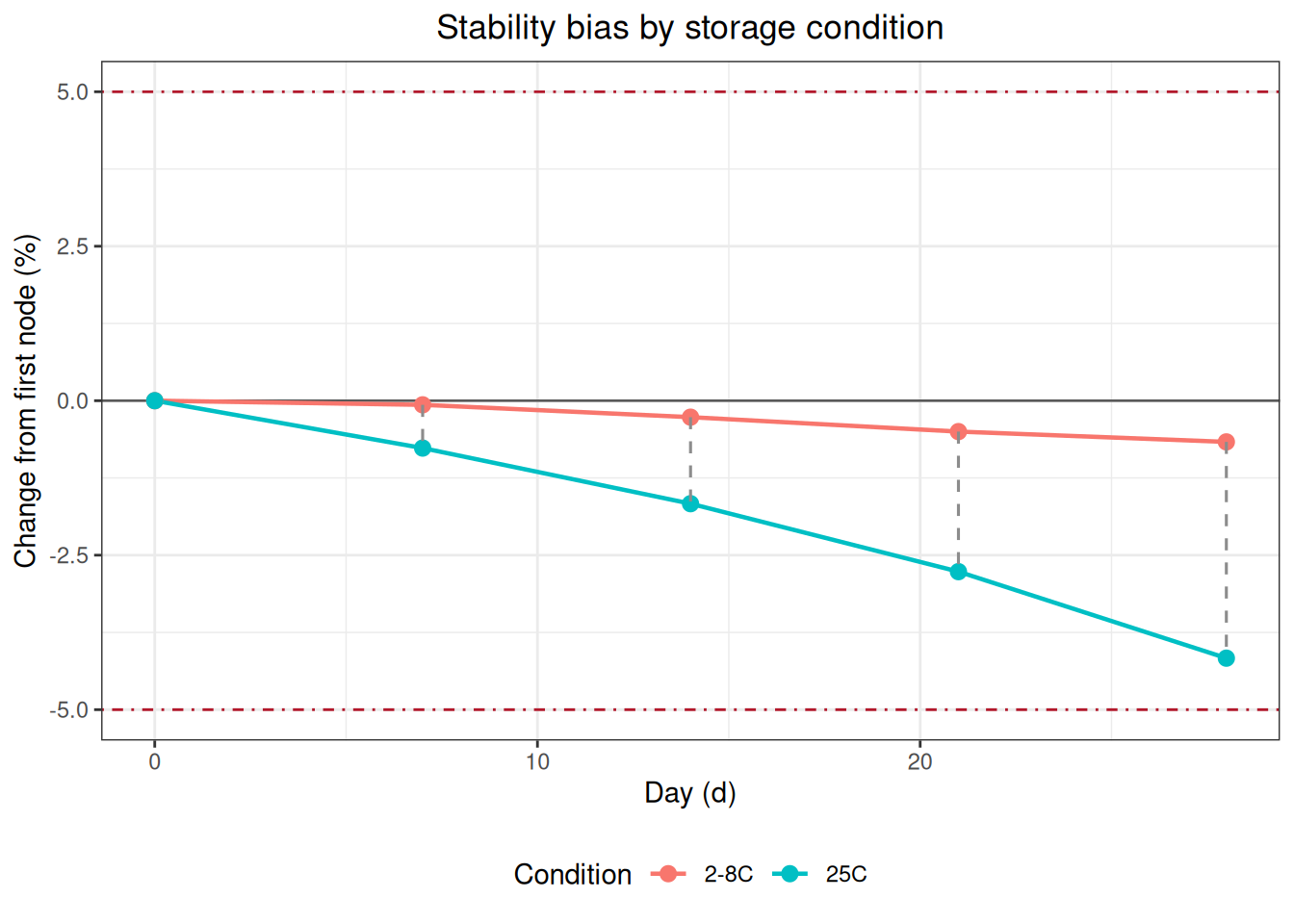

4.1.3 不同保存条件比较的回归分析 `stability_regression()`

读取原始数据：

代码

regression_data <- read_csv(
  "./data/004-稳定性研究/stability-regression-example.csv",
  show_col_types = FALSE
)
head(regression_data, 6)

# A tibble: 6 × 4
  Condition   Day Replicate Result
  <chr>     <dbl>     <dbl>  <dbl>
1 2-8C          0         1  100. 
2 2-8C          0         2   99.9
3 2-8C          0         3  100  
4 2-8C          7         1  100  
5 2-8C          7         2   99.8
6 2-8C          7         3  100.

在每个匹配时间点计算 25C 相对 2-8C 的相对偏差，并对偏差随时间进行回归。示例预先指定结果随时间降低，因此使用 direction = "decrease"。

代码

regression_result <- stability_regression(
  data = regression_data,
  time = "Day",
  value = "Result",
  condition = "Condition",
  mode = "compare",
  test_condition = "25C",
  reference_condition = "2-8C",
  bias_type = "relative",
  direction = "decrease",
  conf.level = 0.95,
  limit = 5,
  time_unit = "d"
)
print(regression_result)


Stability Regression
  Mode:            compare
  Test condition:  25C
  Reference:       2-8C
  Fit:             WLS (1/SE^2); intercept = 0.0799, slope = -0.1025
  Direction:       decrease
  One-sided CI:    95.0%
  R-squared:       0.9956
  Cook distance:   row(s) 6 > 1; not removed

      Time      ObsBias   Estimate   CI_limit Status
  --------------------------------------------------
    0.0000       0.0000     0.0799    -0.0750       
    7.0000      -0.6669    -0.6376    -0.7566       
   14.0000      -1.3013    -1.3552    -1.4522       
   21.0000      -2.0040    -2.0728    -2.1717       
   28.0000      -2.6747    -2.7904    -2.9140       
   42.0000      -4.3842    -4.2256    -4.4296

mode = "self" 用单条件首节点作为参考；mode = "compare" 比较试验条件和参考条件。direction = "auto" 由斜率推断方向，正式方案应尽量显式写成 decrease 或 increase。limit = NULL 只计算模型，不给出接受性状态。

返回 stability_regression，重点字段包括拟合对象、斜率/截距、方向、偏差尺度、置信限、观测时间范围、条件映射和排除记录。用 print() 查看摘要，用 plot() 查看趋势、偏差和置信限。

代码

plot(regression_result)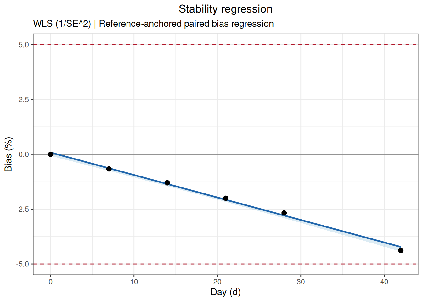

本示例识别出一个 Cook 距离较大的节点，但函数不会自动删除；应回查原始记录、实验过程和方案规定，并在有充分理由时进行包含/不包含该节点的敏感性分析。

4.1.4 与首节点比较的回归分析 `stability_regression()`

mode = "self" 可分析单个条件自身随时间的变化。以下仍使用回归示例数据，但仅选择 25C 条件；各节点的 observed_bias 相对于该条件首节点均值计算：

代码

self_regression_result <- stability_regression(
  data = regression_data,
  time = "Day",
  value = "Result",
  condition = "Condition",
  mode = "self",
  test_condition = "25C",
  bias_type = "relative",
  direction = "decrease",
  conf.level = 0.95,
  limit = 5,
  time_unit = "d"
)
print(self_regression_result)


Stability Regression
  Mode:            self
  Test condition:  25C
  Fit:             WLS (1/SE^2); intercept = 100.0849, slope = -0.1115
  Direction:       decrease
  One-sided CI:    95.0%
  R-squared:       0.9966
  Cook distance:   row(s) 1, 6 > 1; not removed

      Time      ObsBias   Estimate   CI_limit Status
  --------------------------------------------------
    0.0000       0.0000    -0.0000    -0.0000       
    7.0000      -0.7000    -0.7797    -0.8278       
   14.0000      -1.4000    -1.5594    -1.6555       
   21.0000      -2.2000    -2.3391    -2.4833       
   28.0000      -2.9667    -3.1188    -3.3110       
   42.0000      -4.7667    -4.6782    -4.9665

代码

plot(self_regression_result)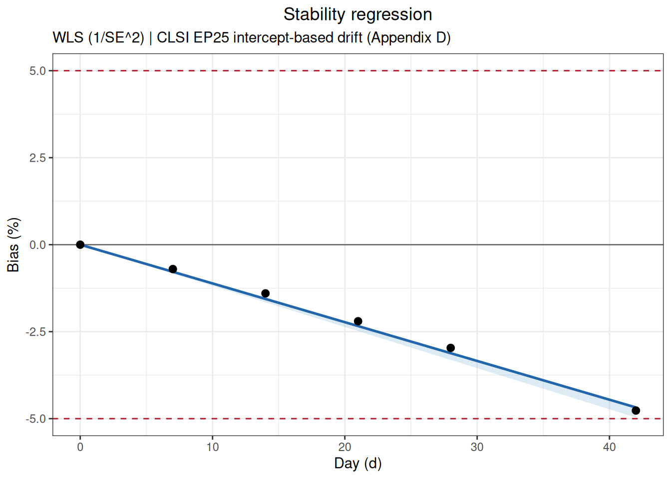

首节点观测偏差固定为 0；模型估计值则由全部时间点共同拟合，不要求回归截距恰好通过首节点。

4.1.5 预测达到限值的时间 `stability_time()`

stability_time() 分别计算点估计和单侧置信限首次达到 -5% 偏差的时间：

代码

time_result <- stability_time(
  regression_result,
  limit = 5,
  max_time = 90
)
print(time_result)


Stability Limit Time
  Limit: 5.0000 (relative); direction: decrease
  estimate       49.5548 d [EXTRAPOLATED]
  one_sided_ci   47.2316 d [EXTRAPOLATED]

输入必须是 stability_regression 对象。函数分别考察点估计或单侧置信限首次达到限值的时间，返回 stability_time，并标记是否超出观测范围。max_time 只是搜索上限，不是科学上合理的货架期；严重外推必须单独论证。

代码

plot(time_result)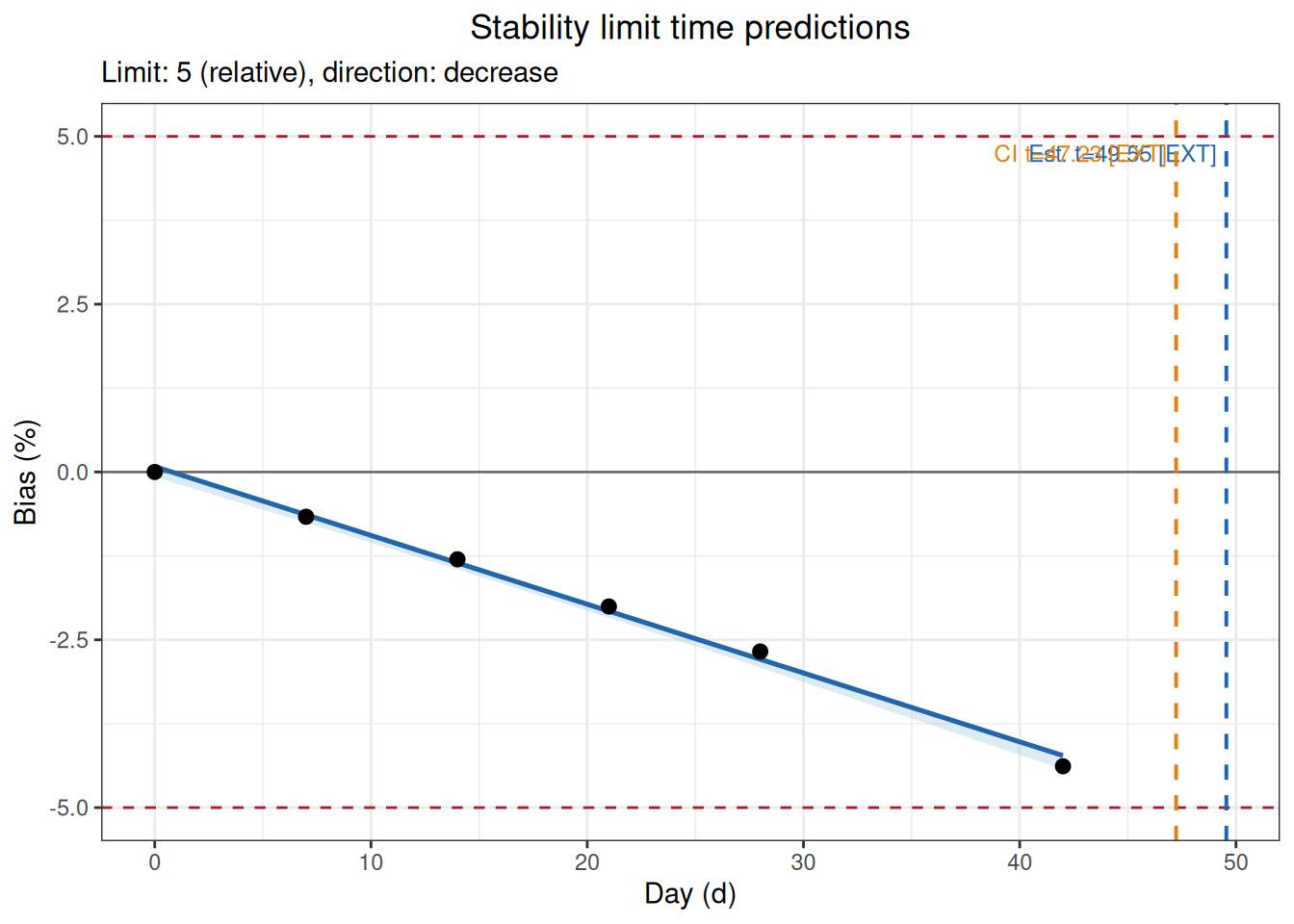

本例最长实际观察时间为 42 天，而预测达到限值的时间超过了观察范围，因此输出标记为 EXTRAPOLATED。外推结果依赖线性趋势在未观察区间继续成立的假设，不能等同于实测稳定性证据；应显著报告外推距离和不确定性，并优先用更长的实际观察数据确认。

4.1.6 阿伦纽斯（Arrhenius）加速稳定性分析 `arrhenius()`

读取和核验原始数据：

代码

arrhenius_data <- read_csv(
  "./data/004-稳定性研究/stability-arrhenius-example.csv",
  show_col_types = FALSE
)
head(arrhenius_data, 6)

# A tibble: 6 × 4
  Temperature   Day Replicate Result
        <dbl> <dbl>     <dbl>  <dbl>
1          30     0         1  100. 
2          30     0         2   99.8
3          30     7         1   99.6
4          30     7         2   99.4
5          30    14         1   99.1
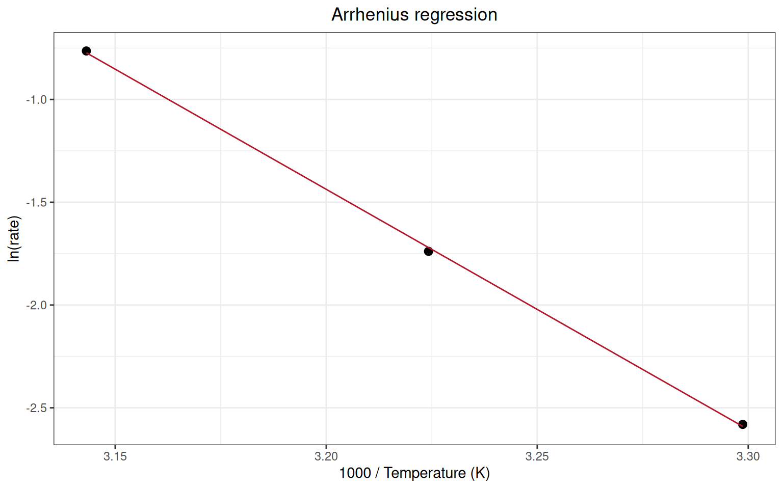
6          30    14         2   98.9

示例使用 30、37 和 45 °C 的加速数据，外推至 5 °C；允许相对变化 10%，并预先指定降解方向为降低：

代码

arrhenius_result <- arrhenius(
  data = arrhenius_data,
  temperature = "Temperature",
  time = "Day",
  value = "Result",
  target_temp = 5,
  order = "auto",
  direction = "decrease",
  limit = 10,
  bias_type = "relative",
  temp_unit = "C",
  time_unit = "d",
  conf.level = 0.95
)
print(arrhenius_result)


Arrhenius Stability Analysis
  Kinetic order:   zero (auto-selected)
  Direction:       decrease
  Activation Ea:   97.159 kJ/mol
  Target rate:     0.002346 /d
  Limit time:      4263.7878 d [1585.3589, 11467.3633]

order 可选 auto、zero、first；temp_unit 可用 C 或 K。返回 arrhenius，包含不同温度的降解速率、活化能、动力学级数、目标温度预测和限值时间。必须检查速率方向、温度覆盖、模型拟合和目标温度外推；不能因 auto 返回结果就视为动力学级数已被验证。从升高温度外推至目标储存温度可能跨越很大范围，预测稳定期及其区间必须与模型假设、实际时间数据和验证研究一起解释。

代码

plot(arrhenius_result)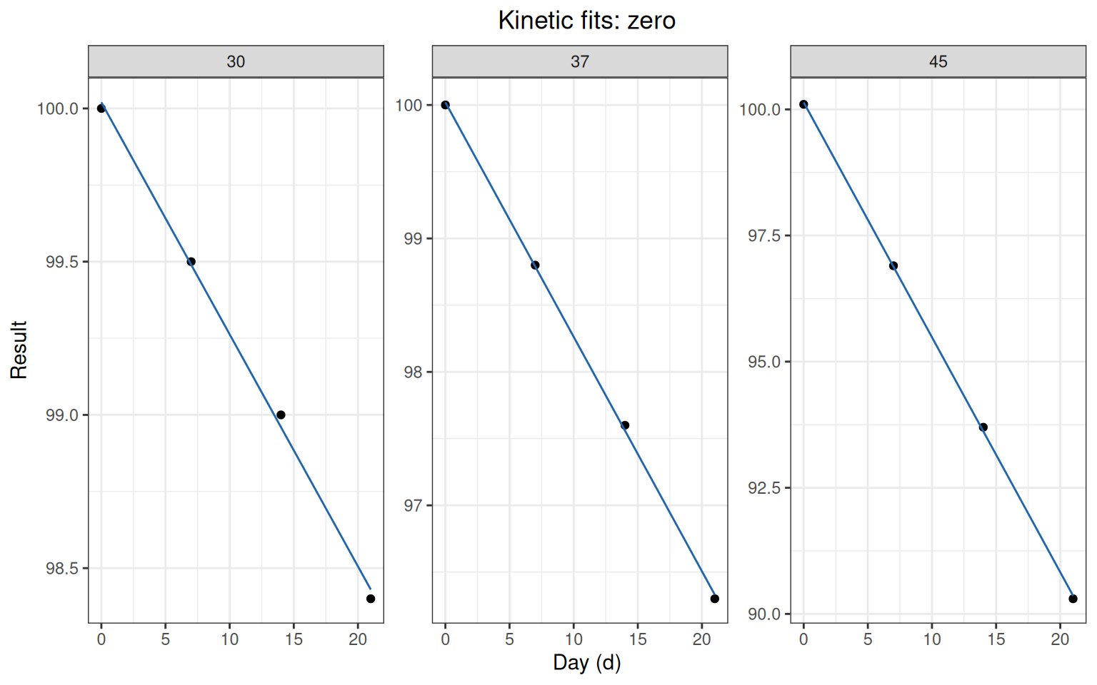

4.1.7 MKT 计算 `mkt()`

读取和核验原始温度数据：

代码

mkt_data <- read_csv(
  "./data/004-稳定性研究/stability-mkt-example.csv",
  show_col_types = FALSE
)
mkt_data$Timestamp <- as.POSIXct(
  mkt_data$Timestamp,
  format = "%Y-%m-%d %H:%M:%S",
  tz = "UTC"
)
head(mkt_data, 6)

# A tibble: 6 × 3
  Timestamp           Probe_A Probe_B
  <dttm>                <dbl>   <dbl>
1 2026-07-01 00:00:00      25    24.5
2 2026-07-01 06:00:00      26    25.5
3 2026-07-01 12:00:00      29    28.5
4 2026-07-01 18:00:00      28    27.5
5 2026-07-02 00:00:00      25    24.8
6 2026-07-02 08:00:00      24    24.2

使用两个温度探头和实际时间间隔，温度单位为摄氏度，活化能采用示例值 83.144 kJ/mol：

代码

mkt_result <- mkt(
  data = mkt_data,
  temp_cols = c("Probe_A", "Probe_B"),
  time = "Timestamp",
  temp_unit = "C",
  ea = 83.144
)
print(mkt_result)


Mean Kinetic Temperature
  Ea: 83.144 kJ/mol
  Method: Time-weighted trapezoidal MKT

  Probe_A              299.538 K     26.388 C
  Probe_B              299.194 K     26.044 C
  Combined             299.367 K     26.217 C

返回 mkt，包含各探头和合并的平均动力学温度。提供 time 时按时间间隔加权；不提供时按等间隔处理。ea 为 kJ/mol 的活化能假设，不能在报告中省略。

4.1.8 多样本数据（长表）拆分

当不同浓度水平、样本类型或批次需要分别评价时，应保留样本标识，先拆分数据，再对每个样本使用相同且预先规定的参数分析。读取并核验多样本原始数据：

代码

multiple_samples_data <- read_csv(
  "./data/004-稳定性研究/stability-multiple-samples-example.csv",
  show_col_types = FALSE
)
head(multiple_samples_data, 6)

# A tibble: 6 × 4
  Sample     Day Replicate Result
  <chr>    <dbl>     <dbl>  <dbl>
1 Sample_A     0         1  100. 
2 Sample_A     0         2   99.8
3 Sample_A     0         3  100  
4 Sample_A     7         1   99.7
5 Sample_A     7         2   99.5
6 Sample_A     7         3   99.8

使用 split_by_factors() 按分类列建立具名数据列表。函数保留拆分列，列表名称直接采用实际样本值，并报告每组行数和因分组缺失而排除的行数：

代码

sample_data_list <- split_by_factors(
  multiple_samples_data,
  variable = "Sample"
)
sample_data_list


Data split by factors
  Variable: Sample
  Groups: 2
  Missing/excluded: 0

  Sample_A  n = 18
  Sample_B  n = 18

代码

sample_a_data <- sample_data_list[["Sample_A"]]

再逐个样本执行分析。

4.2 分析案例

4.2.1 CLSI EP25-A2 附录 B 阿伦纽斯加速稳定性

附录 B 给出控制品在 40、45、50 和 55 ℃下的加速稳定性数据，目标储存温度为 25 ℃，允许结果下降 20%。标准先对各温度的结果取自然对数并拟合一级动力学，再用阿伦纽斯模型外推 25 ℃ 的反应速率和稳定期。

读取和核验原始数据：

代码

ep25_b_data <- read_csv(
  "./data/004-稳定性研究/std-ep25-appendix-b.csv",
  show_col_types = FALSE
)
head(ep25_b_data, 6)

# A tibble: 6 × 3
  Temperature   Day Result
        <dbl> <dbl>  <dbl>
1          40     0  1.02 
2          40    10  0.956
3          40    21  0.945
4          40    31  0.933
5          40    42  0.908
6          40    52  0.86

按标准附录 B 的一级动力学、下降方向、20%允许变化和 25 ℃目标温度进行分析：

代码

ep25_b_result <- arrhenius(
  data = ep25_b_data,
  temperature = "Temperature",
  time = "Day",
  value = "Result",
  target_temp = 25,
  order = "first",
  direction = "decrease",
  limit = 20,
  bias_type = "relative",
  temp_unit = "C",
  time_unit = "d",
  conf.level = 0.95
)
print(ep25_b_result)


Arrhenius Stability Analysis
  Kinetic order:   first
  Direction:       decrease
  Activation Ea:   80.160 kJ/mol
  Target rate:     0.000582 /d
  Limit time:      383.1423 d [330.8315, 443.7244]
  WARNING:         Observed degradation exceeds 20% at one or more temperatures.

代码

plot(ep25_b_result)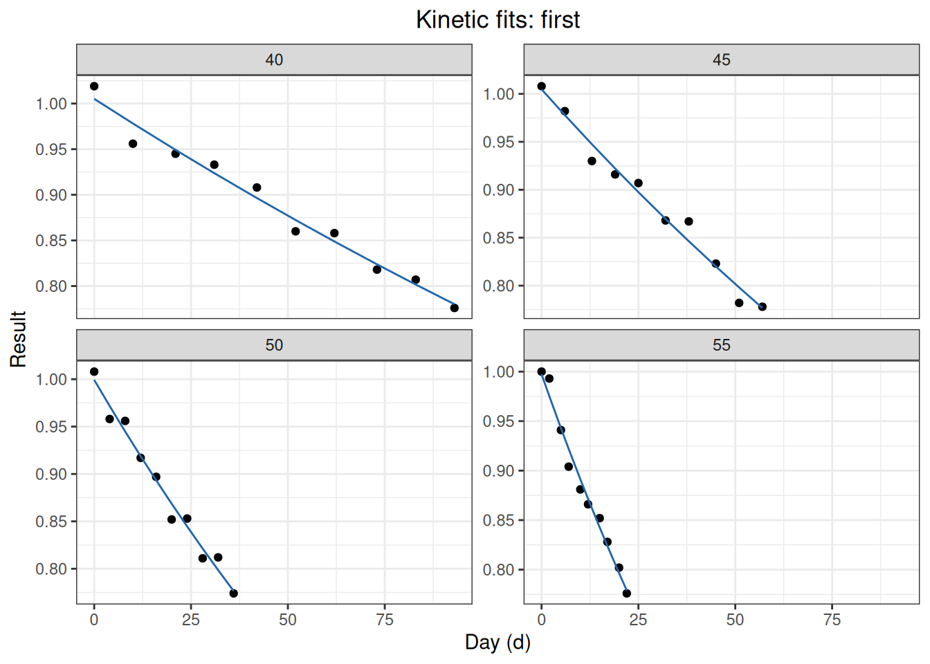

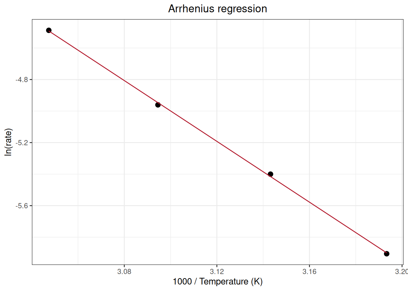
从 arrhenius() 返回对象中提取各温度的降解速率、阿伦纽斯回归系数、25 ℃目标速率和稳定期，再与附录 B 的原文结果对照：

EP25 附录 B：ivdtools 与标准原文结果对照
appendix	statistic	standard	ivdtools
EP25-A2 Appendix B / 40C	rate	2.7257e-03	0.0027257
EP25-A2 Appendix B / 45C	rate	4.5154e-03	0.0045154
EP25-A2 Appendix B / 50C	rate	7.0087e-03	0.0070087
EP25-A2 Appendix B / 55C	rate	1.1243e-02	0.0112430
EP25-A2 Appendix B / Arrhenius	slope	-9.6320e+03	-9640.9966367
EP25-A2 Appendix B / Arrhenius	intercept	2.4874e+01	24.8877147
EP25-A2 Appendix B / 25C	target_rate	5.8250e-04	0.0005824
EP25-A2 Appendix B / 25C	shelf_life	3.8300e+02	383.1423039

4.2.2 CLSI EP25-A2 附录 C1 试剂稳定性

附录 C1 的单批试剂数据覆盖 0～418 天，目标声明期为 364 天，允许漂移为 10%。三个系列均为每个时间点的均值；这里直接按 stability_regression() 的单条件、相对偏差和下降方向处理。

代码

ep25_c1 <- read_csv(
  "./data/004-稳定性研究/std-ep25-appendix-c1.csv",
  show_col_types = FALSE
)
head(ep25_c1, 6)

# A tibble: 6 × 3
  series      day result
  <chr>     <dbl>  <dbl>
1 low_panel     0   7.07
2 low_panel    33   6.95
3 low_panel    61   6.99
4 low_panel    95   6.88
5 low_panel   121   6.98
6 low_panel   155   6.83

代码

ep25_c1_list <- split_by_factors(
  ep25_c1,
  variable = "series"
)
ep25_c1_list


Data split by factors
  Variable: series
  Groups: 3
  Missing/excluded: 0

  low_panel     n = 13
  low_control   n = 13
  high_control  n = 13

使用 stability_regression 进行分析：

代码

ep25_low_panel <- stability_regression(
  ep25_c1_list$low_panel,
  time = "day", value = "result", mode = "self",
  bias_type = "relative", direction = "decrease",
  conf.level = 0.95, limit = 10, time_unit = "d"
)

ep25_low_control <- stability_regression(
  ep25_c1_list$low_control,
  time = "day", value = "result", mode = "self",
  bias_type = "relative", direction = "decrease",
  conf.level = 0.95, limit = 10, time_unit = "d"
)

ep25_high_control <- stability_regression(
  ep25_c1_list$high_control,
  time = "day", value = "result", mode = "self",
  bias_type = "relative", direction = "decrease",
  conf.level = 0.95, limit = 10, time_unit = "d"
)

将计算结果与标准原文结果比较：

EP25 附录 C1：ivdtools 与标准原文结果对照
appendix	statistic	standard	ivdtools
EP25-A2 Appendix C1 / low_panel	slope	-0.001567	-0.001567
EP25-A2 Appendix C1 / low_panel	intercept	7.065000	7.065100
EP25-A2 Appendix C1 / low_panel	change_364	-8.070000	-8.074378
EP25-A2 Appendix C1 / low_panel	change_364_upper_CL	-9.260000	-9.262841
EP25-A2 Appendix C1 / low_panel	change_418	-9.270000	-9.272226
EP25-A2 Appendix C1 / low_panel	change_418_upper_CL	-10.640000	-10.636999
EP25-A2 Appendix C1 / low_control	slope	-0.002873	-0.002873
EP25-A2 Appendix C1 / low_control	intercept	25.270000	25.268365
EP25-A2 Appendix C1 / low_control	change_364	-4.140000	-4.139278
EP25-A2 Appendix C1 / low_control	change_364_upper_CL	-5.130000	-5.129081
EP25-A2 Appendix C1 / low_control	change_418	-4.750000	-4.753346
EP25-A2 Appendix C1 / low_control	change_418_upper_CL	-5.890000	-5.889988
EP25-A2 Appendix C1 / high_control	slope	-0.009103	-0.009103
EP25-A2 Appendix C1 / high_control	intercept	99.740000	99.742806
EP25-A2 Appendix C1 / high_control	change_364	-3.320000	-3.321944
EP25-A2 Appendix C1 / high_control	change_364_upper_CL	-4.170000	-4.166660
EP25-A2 Appendix C1 / high_control	change_418	-3.810000	-3.814759
EP25-A2 Appendix C1 / high_control	change_418_upper_CL	-4.780000	-4.784791

4.2.3 CLSI EP25-A2 附录 C2.1 校准品稳定性（参考锚定实时研究）

比例漂移是分析定义，读取后按 on_test / reference 明确计算，再按水平拆分：

代码

ep25_c2_1_data <- read_csv(
  "./data/004-稳定性研究/std-ep25-appendix-c2-1.csv",
  show_col_types = FALSE
)
head(ep25_c2_1_data, 6)

# A tibble: 6 × 4
  level month on_test reference
  <chr> <dbl>   <dbl>     <dbl>
1 low       0   1.01       1.00
2 low       1   0.999      1.00
3 low       2   0.992      1.01
4 low       4   0.983      1.00
5 low       5   0.985      1.01
6 low       6   0.97       1.00

代码

ep25_c2_1_data$proportional_drift <-
  ep25_c2_1_data$on_test / ep25_c2_1_data$reference
ep25_c2_1_list <- split_by_factors(
  ep25_c2_1_data,
  variable = "level"
)
ep25_c2_1_list


Data split by factors
  Variable: level
  Groups: 2
  Missing/excluded: 0

  low    n = 7
  high   n = 7

使用 stability_regression() 顺序分析两个校准水平：

代码

ep25_c2_1_low_result <- stability_regression(
  data = ep25_c2_1_list$low,
  time = "month",
  value = "proportional_drift",
  mode = "self",
  bias_type = "relative",
  direction = "decrease",
  limit = 5,
  time_unit = "month",
  conf.level = 0.95
)

ep25_c2_1_high_result <- stability_regression(
  data = ep25_c2_1_list$high,
  time = "month",
  value = "proportional_drift",
  mode = "self",
  bias_type = "relative",
  direction = "decrease",
  limit = 5,
  time_unit = "month",
  conf.level = 0.95
)

ep25_c2_1_low_time <- stability_time(
  ep25_c2_1_low_result,
  max_time = 20
)
ep25_c2_1_high_time <- stability_time(
  ep25_c2_1_high_result,
  max_time = 20
)

print(ep25_c2_1_low_result)


Stability Regression
  Mode:            self
  Test condition:  condition
  Fit:             OLS; intercept = 1.0020, slope = -0.0059
  Direction:       decrease
  One-sided CI:    95.0%
  R-squared:       0.9566
  Cook distance:   row(s) 1 > 1; not removed
  Note:            WLS unavailable; OLS used.

      Time      ObsBias   Estimate   CI_limit Status
  --------------------------------------------------
    0.0000       0.0000    -0.0000    -0.0000       
    1.0000      -1.2873    -0.5887    -0.6995       
    2.0000      -2.1737    -1.1775    -1.3989       
    4.0000      -2.8683    -2.3549    -2.7978       
    5.0000      -3.2483    -2.9437    -3.4973       
    6.0000      -3.8659    -3.5324    -4.1968       
    6.5000      -4.3541    -3.8268    -4.5465

代码

print(ep25_c2_1_high_result)


Stability Regression
  Mode:            self
  Test condition:  condition
  Fit:             OLS; intercept = 1.0078, slope = -0.0054
  Direction:       decrease
  One-sided CI:    95.0%
  R-squared:       0.5652
  Cook distance:   row(s) 7 > 1; not removed
  Note:            WLS unavailable; OLS used.

      Time      ObsBias   Estimate   CI_limit Status
  --------------------------------------------------
    0.0000       0.0000    -0.0000    -0.0000       
    1.0000       0.2612    -0.5317    -0.9441       
    2.0000      -0.0475    -1.0633    -1.8881       
    4.0000      -0.3329    -2.1266    -3.7763       
    5.0000      -2.2787    -2.6583    -4.7204       
    6.0000      -0.8759    -3.1900    -5.6644      *
    6.5000      -4.7539    -3.4558    -6.1365      *

代码

plot(ep25_c2_1_low_result)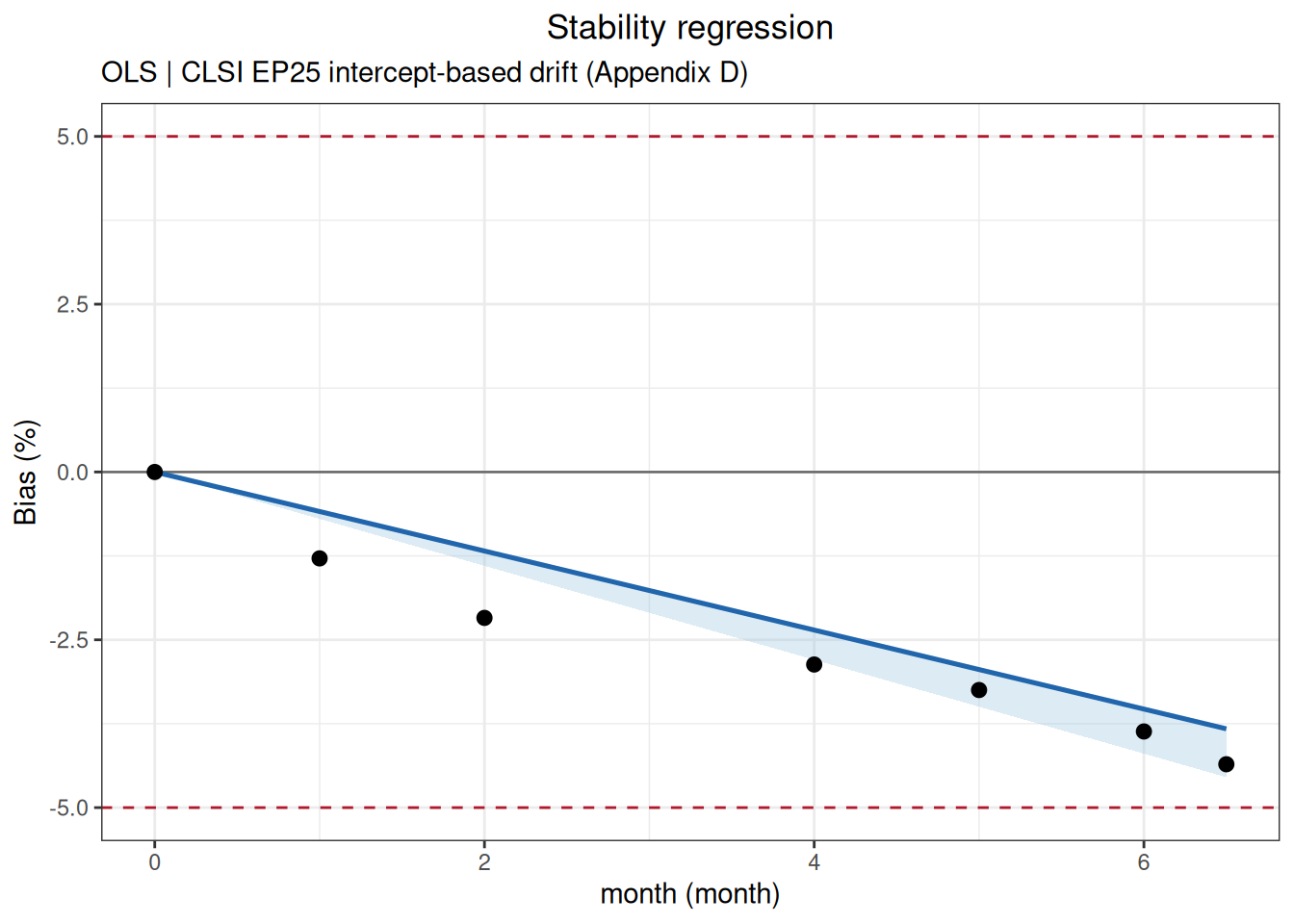

代码

plot(ep25_c2_1_high_result)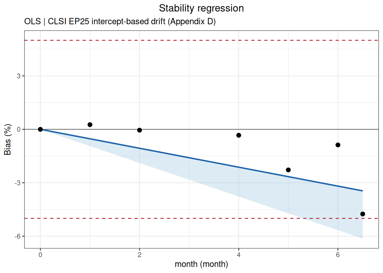

与标准原文结果比较：

EP25 附录 C2.1：ivdtools 与标准原文结果对照
appendix	statistic	standard	ivdtools
EP25-A2 Appendix C2.1 / low_calibrator	change_6	-3.53	-3.532421
EP25-A2 Appendix C2.1 / low_calibrator	change_6_upper_CL	-4.20	-4.196768
EP25-A2 Appendix C2.1 / low_calibrator	change_6.5	-3.83	-3.826789
EP25-A2 Appendix C2.1 / low_calibrator	change_6.5_upper_CL	-4.55	-4.546498
EP25-A2 Appendix C2.1 / low_calibrator	ci_limit_time	7.10	7.148359
EP25-A2 Appendix C2.1 / high_calibrator	change_6	-3.19	-3.189971
EP25-A2 Appendix C2.1 / high_calibrator	change_6_upper_CL	-5.66	-5.664441
EP25-A2 Appendix C2.1 / high_calibrator	change_6.5	-3.46	-3.455801
EP25-A2 Appendix C2.1 / high_calibrator	change_6.5_upper_CL	-6.14	-6.136478
EP25-A2 Appendix C2.1 / high_calibrator	ci_limit_time	5.30	5.296198

4.2.4 CLSI EP25-A2 附录 C2.2 校准品稳定性（等时研究）

代码

ep25_c2_2_data <- read_csv(
  "./data/004-稳定性研究/std-ep25-appendix-c2-2.csv",
  show_col_types = FALSE
)
head(ep25_c2_2_data, 6)

# A tibble: 6 × 3
  level     day result
  <chr>   <dbl>  <dbl>
1 level_1     0   19.9
2 level_1    15   20.2
3 level_1    31   20.2
4 level_1    62   20.3
5 level_1    94   20.7
6 level_1   123   21.1

代码

ep25_c2_2_list <- split_by_factors(
  ep25_c2_2_data,
  variable = "level"
)
ep25_c2_2_list


Data split by factors
  Variable: level
  Groups: 3
  Missing/excluded: 0

  level_1  n = 9
  level_2  n = 9
  level_3  n = 9

使用 stability_regression() 顺序分析三个校准水平：

代码

ep25_c2_2_level_1_result <- stability_regression(
  data = ep25_c2_2_list$level_1,
  time = "day",
  value = "result",
  mode = "self",
  bias_type = "relative",
  direction = "increase",
  limit = 10,
  time_unit = "d",
  conf.level = 0.95
)

ep25_c2_2_level_2_result <- stability_regression(
  data = ep25_c2_2_list$level_2,
  time = "day",
  value = "result",
  mode = "self",
  bias_type = "relative",
  direction = "increase",
  limit = 10,
  time_unit = "d",
  conf.level = 0.95
)

ep25_c2_2_level_3_result <- stability_regression(
  data = ep25_c2_2_list$level_3,
  time = "day",
  value = "result",
  mode = "self",
  bias_type = "relative",
  direction = "increase",
  limit = 10,
  time_unit = "d",
  conf.level = 0.95
)

print(ep25_c2_2_level_1_result)


Stability Regression
  Mode:            self
  Test condition:  condition
  Fit:             OLS; intercept = 19.9291, slope = 0.0088
  Direction:       increase
  One-sided CI:    95.0%
  R-squared:       0.9789
  Note:            WLS unavailable; OLS used.

      Time      ObsBias   Estimate   CI_limit Status
  --------------------------------------------------
    0.0000       0.0000     0.0000     0.0000       
   15.0000       1.5075     0.6616     0.7341       
   31.0000       1.5075     1.3673     1.5171       
   62.0000       2.0101     2.7345     3.0343       
   94.0000       4.0201     4.1459     4.6003       
  123.0000       6.0302     5.4249     6.0196       
  154.0000       7.0352     6.7922     7.5367       
  180.0000       8.5427     7.9389     8.8092       
  210.0000       9.0452     9.2620    10.2774      *

代码

print(ep25_c2_2_level_2_result)


Stability Regression
  Mode:            self
  Test condition:  condition
  Fit:             OLS; intercept = 100.9678, slope = 0.0292
  Direction:       increase
  One-sided CI:    95.0%
  R-squared:       0.9426
  Note:            WLS unavailable; OLS used.

      Time      ObsBias   Estimate   CI_limit Status
  --------------------------------------------------
    0.0000       0.0000     0.0000     0.0000       
   15.0000       1.2859     0.4341     0.5129       
   31.0000       0.3956     0.8970     1.0600       
   62.0000       0.9891     1.7941     2.1201       
   94.0000       2.3739     2.7201     3.2143       
  123.0000       2.9674     3.5592     4.2060       
  154.0000       4.1543     4.4563     5.2660       
  180.0000       5.7369     5.2087     6.1551       
  210.0000       6.0336     6.0768     7.1809

代码

print(ep25_c2_2_level_3_result)


Stability Regression
  Mode:            self
  Test condition:  condition
  Fit:             OLS; intercept = 502.3132, slope = 0.2573
  Direction:       increase
  One-sided CI:    95.0%
  R-squared:       0.9808
  Note:            WLS unavailable; OLS used.

      Time      ObsBias   Estimate   CI_limit Status
  --------------------------------------------------
    0.0000       0.0000     0.0000     0.0000       
   15.0000       0.9014     0.7683     0.8491       
   31.0000       2.8045     1.5878     1.7547       
   62.0000       4.5873     3.1756     3.5094       
   94.0000       5.6691     4.8147     5.3207       
  123.0000       7.2516     6.3001     6.9622       
  154.0000       8.2332     7.8879     8.7169       
  180.0000       9.2147     9.2196    10.1886      *
  210.0000      11.7388    10.7562    11.8867      *

代码

plot(ep25_c2_2_level_3_result)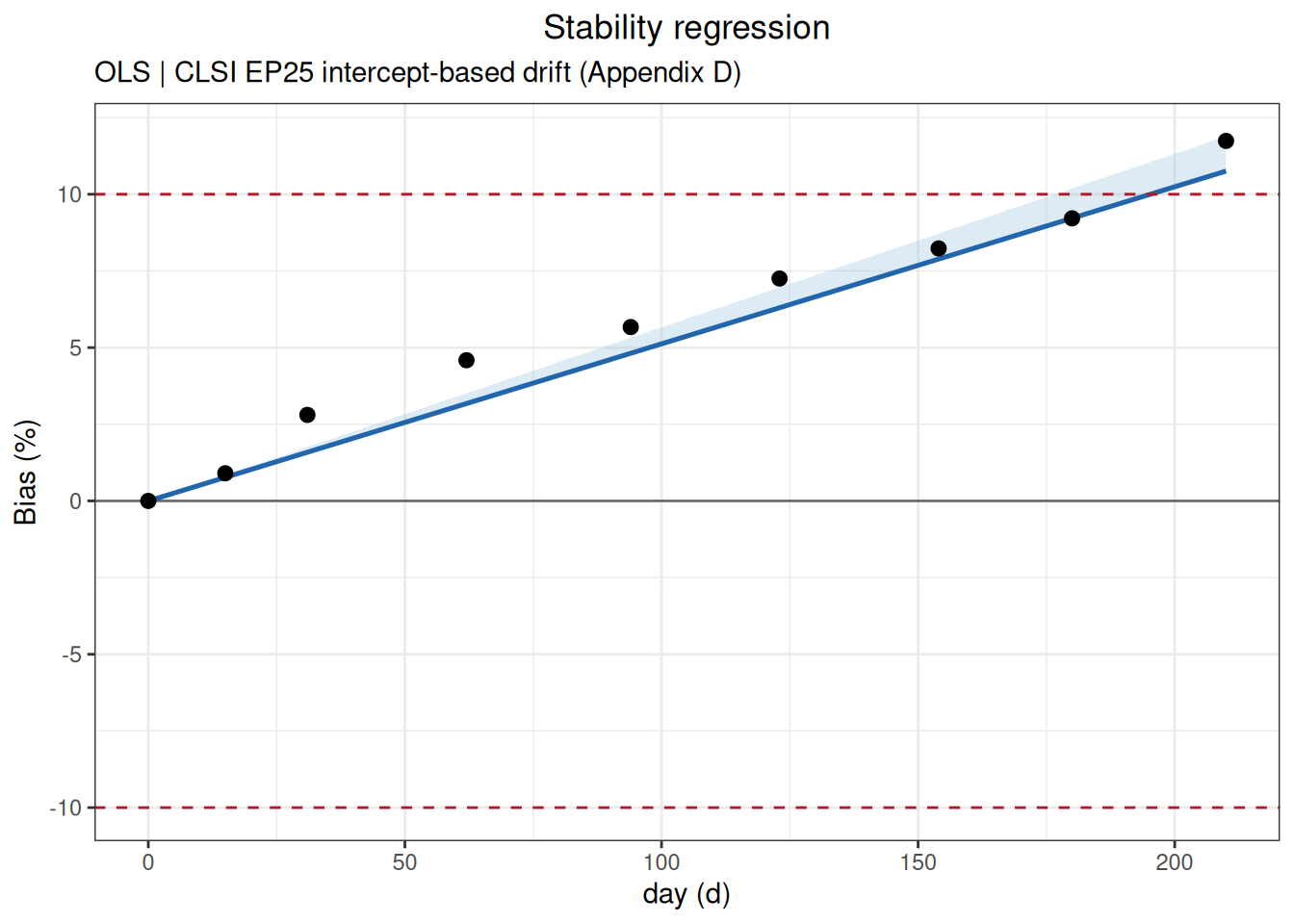

与标准原文结果比较：

EP25 附录 C2.2：ivdtools 与标准原文结果对照
appendix	statistic	standard	ivdtools
EP25-A2 Appendix C2.2 / level_1	change_180	7.97	7.938892
EP25-A2 Appendix C2.2 / level_1	change_180_upper_CL	8.78	8.809166
EP25-A2 Appendix C2.2 / level_1	change_210	9.30	9.262041
EP25-A2 Appendix C2.2 / level_1	change_210_upper_CL	10.24	10.277360
EP25-A2 Appendix C2.2 / level_2	change_180	5.19	5.208658
EP25-A2 Appendix C2.2 / level_2	change_180_upper_CL	6.11	6.155086
EP25-A2 Appendix C2.2 / level_2	change_210	6.05	6.076767
EP25-A2 Appendix C2.2 / level_2	change_210_upper_CL	7.13	7.180933
EP25-A2 Appendix C2.2 / level_3	change_180	9.19	9.219626
EP25-A2 Appendix C2.2 / level_3	change_180_upper_CL	10.18	10.188639
EP25-A2 Appendix C2.2 / level_3	change_210	10.73	10.756231
EP25-A2 Appendix C2.2 / level_3	change_210_upper_CL	11.87	11.886745

4.2.5 CLSI EP25-A2 附录 C3.1 控制品稳定性（参考锚定实时研究）

代码

ep25_c3_1_data <- read_csv(
  "./data/004-稳定性研究/std-ep25-appendix-c3-1.csv",
  show_col_types = FALSE
)
head(ep25_c3_1_data, 6)

# A tibble: 6 × 4
  control  month condition result
  <chr>    <dbl> <chr>      <dbl>
1 negative     0 reference   0.23
2 negative     1 reference   0.24
3 negative     2 reference   0.24
4 negative     3 reference   0.23
5 negative     4 reference   0.24
6 negative     5 reference   0.25

代码

ep25_c3_1_list <- split_by_factors(
  ep25_c3_1_data,
  variable = "control"
)
ep25_c3_1_list


Data split by factors
  Variable: control
  Groups: 2
  Missing/excluded: 0

  negative  n = 18
  positive  n = 18

使用 stability_regression() 分别处理阴性和阳性对照：

代码

ep25_c3_1_negative_result <- stability_regression(
  data = ep25_c3_1_list$negative,
  time = "month",
  value = "result",
  condition = "condition",
  mode = "compare",
  test_condition = "on_test",
  reference_condition = "reference",
  bias_type = "absolute",
  direction = "increase",
  limit = 0.10,
  time_unit = "month",
  conf.level = 0.95
)

ep25_c3_1_positive_result <- stability_regression(
  data = ep25_c3_1_list$positive,
  time = "month",
  value = "result",
  condition = "condition",
  mode = "compare",
  test_condition = "on_test",
  reference_condition = "reference",
  bias_type = "relative",
  direction = "decrease",
  limit = 5,
  time_unit = "month",
  conf.level = 0.95
)

print(ep25_c3_1_negative_result)


Stability Regression
  Mode:            compare
  Test condition:  on_test
  Reference:       reference
  Fit:             OLS; intercept = 0.0004, slope = 0.0103
  Direction:       increase
  One-sided CI:    95.0%
  R-squared:       0.8962
  Note:            WLS unavailable; OLS used.

      Time      ObsBias   Estimate   CI_limit Status
  --------------------------------------------------
    0.0000       0.0000     0.0004     0.0121       
    1.0000       0.0200     0.0107     0.0204       
    2.0000       0.0300     0.0210     0.0290       
    3.0000       0.0200     0.0314     0.0381       
    4.0000       0.0300     0.0417     0.0480       
    5.0000       0.0400     0.0520     0.0588       
    6.0000       0.0700     0.0623     0.0705       
    7.0000       0.0800     0.0727     0.0826       
    7.5000       0.0800     0.0778     0.0888

代码

print(ep25_c3_1_positive_result)


Stability Regression
  Mode:            compare
  Test condition:  on_test
  Reference:       reference
  Fit:             OLS; intercept = -0.0461, slope = -0.3655
  Direction:       decrease
  One-sided CI:    95.0%
  R-squared:       0.7765
  Note:            WLS unavailable; OLS used.

      Time      ObsBias   Estimate   CI_limit Status
  --------------------------------------------------
    0.0000      -0.1992    -0.0461    -0.7018       
    1.0000      -0.5988    -0.4116    -0.9539       
    2.0000      -0.8016    -0.7772    -1.2218       
    3.0000      -1.3917    -1.1427    -1.5179       
    4.0000      -1.3972    -1.5082    -1.8593       
    5.0000      -0.8048    -1.8738    -2.2547       
    6.0000      -1.8036    -2.2393    -2.6937       
    7.0000      -2.7944    -2.6048    -3.1591       
    7.5000      -3.6000    -2.7876    -3.3979

代码

plot(ep25_c3_1_negative_result)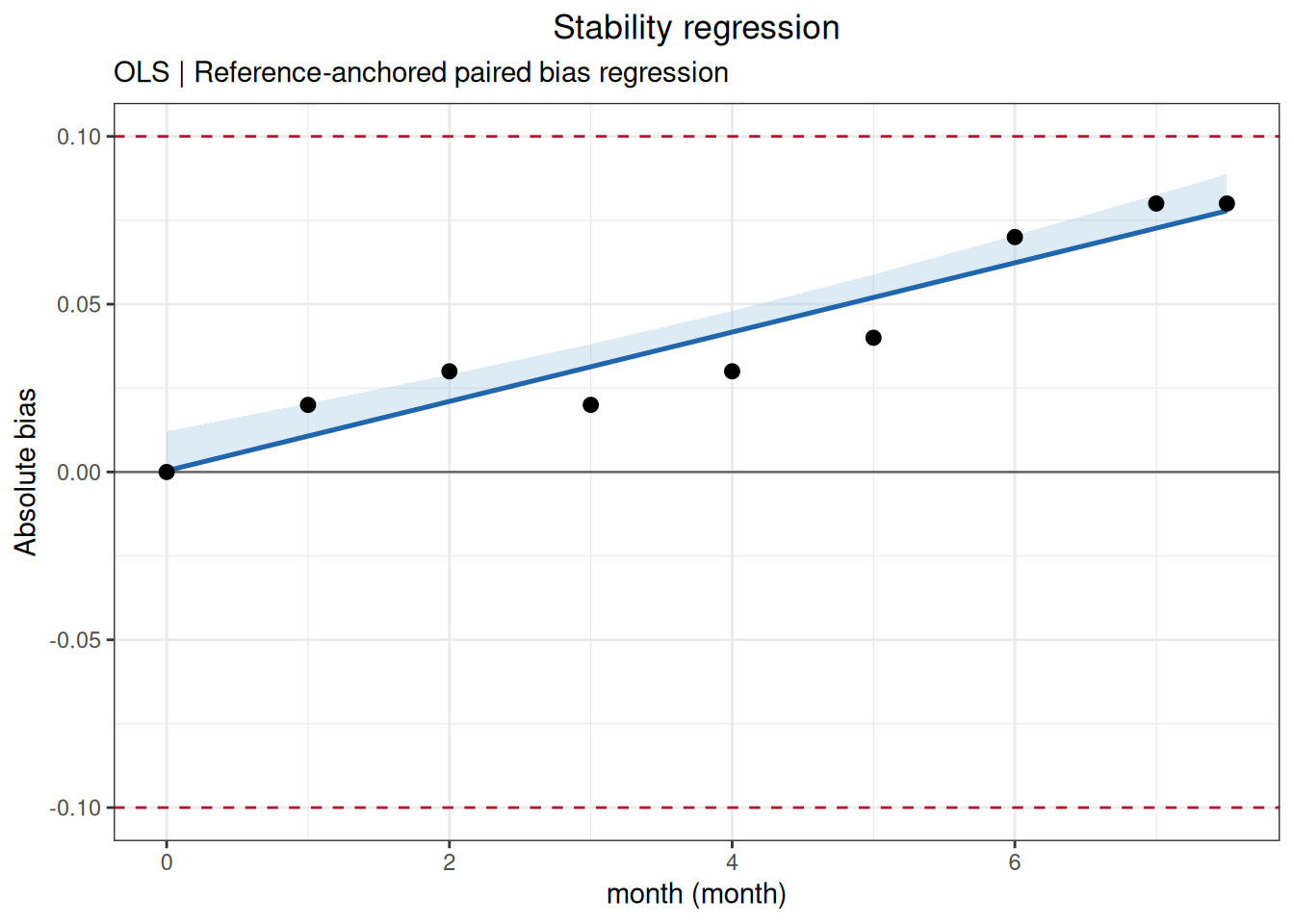

与标准原文结果比较：

EP25 附录 C3.1：ivdtools 与标准原文结果对照
appendix	statistic	standard	ivdtools
EP25-A2 Appendix C3.1 / negative_control	change_7	0.07	0.072663
EP25-A2 Appendix C3.1 / negative_control	change_7_upper_CL	0.09	0.082595
EP25-A2 Appendix C3.1 / negative_control	change_7.5	0.08	0.077826
EP25-A2 Appendix C3.1 / negative_control	change_7.5_upper_CL	0.10	0.088761
EP25-A2 Appendix C3.1 / positive_control	change_7	-2.56	-2.604835
EP25-A2 Appendix C3.1 / positive_control	change_7_upper_CL	-3.53	-3.159133
EP25-A2 Appendix C3.1 / positive_control	change_7.5	-2.74	-2.787602
EP25-A2 Appendix C3.1 / positive_control	change_7.5_upper_CL	-3.79	-3.397864

阴性对照使用绝对偏差和 0.10 IU/mL 限值，阳性对照使用相对偏差和 5% 限值；

4.2.6 CLSI EP25-A2 附录 C3.2 控制品稳定性（等时研究）

代码

ep25_c3_2_data <- read_csv(
  "./data/004-稳定性研究/std-ep25-appendix-c3-2.csv",
  show_col_types = FALSE
)
head(ep25_c3_2_data, 6)

# A tibble: 6 × 3
  level     day result
  <chr>   <dbl>  <dbl>
1 level_1     0   1.21
2 level_1    40   1.17
3 level_1    80   1.22
4 level_1   120   1.18
5 level_1   162   1.15
6 level_1   203   1.14

代码

ep25_c3_2_list <- split_by_factors(
  ep25_c3_2_data,
  variable = "level"
)
ep25_c3_2_list


Data split by factors
  Variable: level
  Groups: 3
  Missing/excluded: 0

  level_1  n = 10
  level_2  n = 10
  level_3  n = 10

使用 stability_regression() 顺序分析三个控制水平：

代码

ep25_c3_2_level_1_result <- stability_regression(
  data = ep25_c3_2_list$level_1,
  time = "day",
  value = "result",
  mode = "self",
  bias_type = "relative",
  direction = "decrease",
  limit = 10,
  time_unit = "d",
  conf.level = 0.95
)

ep25_c3_2_level_2_result <- stability_regression(
  data = ep25_c3_2_list$level_2,
  time = "day",
  value = "result",
  mode = "self",
  bias_type = "relative",
  direction = "decrease",
  limit = 10,
  time_unit = "d",
  conf.level = 0.95
)

ep25_c3_2_level_3_result <- stability_regression(
  data = ep25_c3_2_list$level_3,
  time = "day",
  value = "result",
  mode = "self",
  bias_type = "relative",
  direction = "decrease",
  limit = 10,
  time_unit = "d",
  conf.level = 0.95
)

print(ep25_c3_2_level_1_result)


Stability Regression
  Mode:            self
  Test condition:  condition
  Fit:             OLS; intercept = 1.2060, slope = -0.0003
  Direction:       decrease
  One-sided CI:    95.0%
  R-squared:       0.7575
  Note:            WLS unavailable; OLS used.

      Time      ObsBias   Estimate   CI_limit Status
  --------------------------------------------------
    0.0000       0.0000    -0.0000    -0.0000       
   40.0000      -3.3058    -0.9917    -1.3431       
   80.0000       0.8264    -1.9833    -2.6861       
  120.0000      -2.4793    -2.9750    -4.0292       
  162.0000      -4.9587    -4.0162    -5.4394       
  203.0000      -5.7851    -5.0327    -6.8160       
  255.0000      -8.2645    -6.3219    -8.5620       
  305.0000     -10.7438    -7.5614   -10.2408      *
  364.0000      -6.6116    -9.0241   -12.2218      *
  410.0000      -9.9174   -10.1645   -13.7663      *

代码

print(ep25_c3_2_level_2_result)


Stability Regression
  Mode:            self
  Test condition:  condition
  Fit:             OLS; intercept = 3.4233, slope = -0.0012
  Direction:       decrease
  One-sided CI:    95.0%
  R-squared:       0.9402
  Note:            WLS unavailable; OLS used.

      Time      ObsBias   Estimate   CI_limit Status
  --------------------------------------------------
    0.0000       0.0000    -0.0000    -0.0000       
   40.0000       0.8798    -1.3939    -1.6098       
   80.0000      -2.3460    -2.7879    -3.2195       
  120.0000      -5.5718    -4.1818    -4.8293       
  162.0000      -4.1056    -5.6454    -6.5195       
  203.0000      -6.7449    -7.0742    -8.1695       
  255.0000     -10.2639    -8.8863   -10.2622      *
  305.0000     -11.1437   -10.6287   -12.2744      *
  364.0000     -11.7302   -12.6847   -14.6488      *
  410.0000     -12.9032   -14.2877   -16.5001      *

代码

print(ep25_c3_2_level_3_result)


Stability Regression
  Mode:            self
  Test condition:  condition
  Fit:             OLS; intercept = 7.5028, slope = -0.0016
  Direction:       decrease
  One-sided CI:    95.0%
  R-squared:       0.9912
  Note:            WLS unavailable; OLS used.

      Time      ObsBias   Estimate   CI_limit Status
  --------------------------------------------------
    0.0000       0.0000    -0.0000    -0.0000       
   40.0000      -0.9321    -0.8327    -0.8822       
   80.0000      -1.5979    -1.6653    -1.7645       
  120.0000      -2.6631    -2.4980    -2.6467       
  162.0000      -3.1957    -3.3723    -3.5731       
  203.0000      -4.5273    -4.2258    -4.4774       
  255.0000      -5.8589    -5.3083    -5.6243       
  305.0000      -6.7909    -6.3491    -6.7271       
  364.0000      -7.3236    -7.5773    -8.0285       
  410.0000      -8.3888    -8.5348    -9.0431

代码

plot(ep25_c3_2_level_2_result)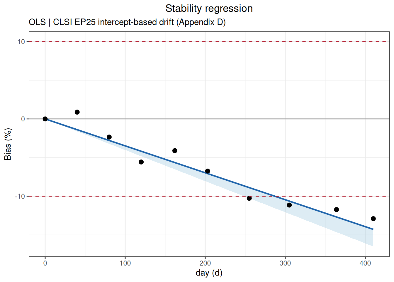

与标准原文结果比较：

EP25 附录 C3.2：ivdtools 与标准原文结果对照
appendix	statistic	standard	ivdtools
EP25-A2 Appendix C3.2 / level_1	change_364	-9.00	-9.024133
EP25-A2 Appendix C3.2 / level_1	change_364_upper_CL	-12.19	-12.221806
EP25-A2 Appendix C3.2 / level_1	change_410	-10.14	-10.164545
EP25-A2 Appendix C3.2 / level_1	change_410_upper_CL	-13.73	-13.766320
EP25-A2 Appendix C3.2 / level_2	change_364	-12.68	-12.684724
EP25-A2 Appendix C3.2 / level_2	change_364_upper_CL	-14.66	-14.648829
EP25-A2 Appendix C3.2 / level_2	change_410	-14.28	-14.287738
EP25-A2 Appendix C3.2 / level_2	change_410_upper_CL	-16.52	-16.500055
EP25-A2 Appendix C3.2 / level_3	change_364	-7.58	-7.577276
EP25-A2 Appendix C3.2 / level_3	change_364_upper_CL	-8.05	-8.028464
EP25-A2 Appendix C3.2 / level_3	change_410	-8.54	-8.534844
EP25-A2 Appendix C3.2 / level_3	change_410_upper_CL	-9.07	-9.043050

三个控制水平均按相对偏差、下降方向和 10% 允许变化处理。结果比较使用函数直接返回的节点估计及单侧置信限。

4.2.7 CLSI EP25-A2 附录 C4 运输条件

代码

ep25_c4_data <- read_csv(
  "./data/004-稳定性研究/std-ep25-appendix-c4.csv",
  show_col_types = FALSE
)
head(ep25_c4_data, 6)

# A tibble: 6 × 5
  sample    condition   time replicate result
  <chr>     <chr>      <dbl>     <dbl>  <dbl>
1 low_panel unstressed     0         1   7.24
2 low_panel unstressed     0         2   6.98
3 low_panel unstressed     0         3   6.94
4 low_panel unstressed     0         4   6.82
5 low_panel unstressed     0         5   7.09
6 low_panel unstressed     0         6   7.14

代码

ep25_c4_list <- split_by_factors(
  ep25_c4_data,
  variable = "sample"
)
ep25_c4_list


Data split by factors
  Variable: sample
  Groups: 3
  Missing/excluded: 0

  low_panel     n = 20
  low_control   n = 20
  high_control  n = 20

使用 stability_bias() 分别评价三个样本：

代码

ep25_c4_low_panel_result <- stability_bias(
  data = ep25_c4_list$low_panel,
  condition = "condition",
  time = "time",
  value = "result",
  reference_condition = "unstressed",
  limit = 5,
  bias_type = "relative",
  time_unit = "d"
)

ep25_c4_low_control_result <- stability_bias(
  data = ep25_c4_list$low_control,
  condition = "condition",
  time = "time",
  value = "result",
  reference_condition = "unstressed",
  limit = 5,
  bias_type = "relative",
  time_unit = "d"
)

ep25_c4_high_control_result <- stability_bias(
  data = ep25_c4_list$high_control,
  condition = "condition",
  time = "time",
  value = "result",
  reference_condition = "unstressed",
  limit = 5,
  bias_type = "relative",
  time_unit = "d"
)

print(ep25_c4_low_panel_result)


Stability Bias Analysis
  Conditions:      2 (unstressed, stressed)
  Reference:       unstressed
  Time unit:       d
  Node comparisons:0
  Acceptance:      +/- 5.0000 (relative); 2/2 nodes passed

  Within-condition bias (vs first node)
  Cond         Time      Value    Bias(%) Status
  ----------------------------------------------
  unstressed   0.0000     7.0710     0.0000 Pass
  stressed   0.0000     7.0700     0.0000 Pass

  Between-condition bias (reference: unstressed)
      Time Condition    TestVal  Bias(%)
  --------------------------------------
    0.0000 stressed     7.0700    -0.0141

代码

print(ep25_c4_low_control_result)


Stability Bias Analysis
  Conditions:      2 (unstressed, stressed)
  Reference:       unstressed
  Time unit:       d
  Node comparisons:0
  Acceptance:      +/- 5.0000 (relative); 2/2 nodes passed

  Within-condition bias (vs first node)
  Cond         Time      Value    Bias(%) Status
  ----------------------------------------------
  unstressed   0.0000    25.1740     0.0000 Pass
  stressed   0.0000    25.1630     0.0000 Pass

  Between-condition bias (reference: unstressed)
      Time Condition    TestVal  Bias(%)
  --------------------------------------
    0.0000 stressed    25.1630    -0.0437

代码

print(ep25_c4_high_control_result)


Stability Bias Analysis
  Conditions:      2 (unstressed, stressed)
  Reference:       unstressed
  Time unit:       d
  Node comparisons:0
  Acceptance:      +/- 5.0000 (relative); 2/2 nodes passed

  Within-condition bias (vs first node)
  Cond         Time      Value    Bias(%) Status
  ----------------------------------------------
  unstressed   0.0000    99.1610     0.0000 Pass
  stressed   0.0000    99.6930     0.0000 Pass

  Between-condition bias (reference: unstressed)
      Time Condition    TestVal  Bias(%)
  --------------------------------------
    0.0000 stressed    99.6930     0.5365

与标准原文结果比较：

EP25 附录 C4：ivdtools 与标准原文结果对照
appendix	statistic	standard	ivdtools
EP25-A2 Appendix C4 / low_panel	relative_bias	0.0	-0.014142
EP25-A2 Appendix C4 / low_control	relative_bias	0.0	-0.043696
EP25-A2 Appendix C4 / high_control	relative_bias	0.5	0.536501

运输条件案例使用 stability_bias() 的参考条件比较结果。标准原文还报告了重复测定的置信区间，但本函数的 between_bias 不返回该项，因此比较表只列出函数直接返回的相对偏差。

4.2.8 CLSI EP25-A2 附录 C5 离群值评价

读取和核验标准数据：

代码

ep25_c5_data <- read_csv(
  "./data/004-稳定性研究/std-ep25-appendix-c5.csv",
  show_col_types = FALSE
)
head(ep25_c5_data, 6)

# A tibble: 6 × 2
    Day Result
  <dbl>  <dbl>
1     0   12.1
2    31   12.0
3    61   15.0
4    96   11.9
5   120   11.8
6   150   11.8

代码

ep25_c5_without_day_61 <- ep25_c5_data[ep25_c5_data$Day != 61, ]
head(ep25_c5_without_day_61, 6)

# A tibble: 6 × 2
    Day Result
  <dbl>  <dbl>
1     0   12.1
2    31   12.0
3    96   11.9
4   120   11.8
5   150   11.8
6   186   11.8

使用 stability_regression() 评价含离群值和剔除离群值的结果:

代码

ep25_c5_with_result <- stability_regression(
  data = ep25_c5_data,
  time = "Day",
  value = "Result",
  mode = "self",
  bias_type = "relative",
  direction = "decrease",
  limit = 10,
  time_unit = "d",
  conf.level = 0.95
)

ep25_c5_without_result <- stability_regression(
  data = ep25_c5_without_day_61,
  time = "Day",
  value = "Result",
  mode = "self",
  bias_type = "relative",
  direction = "decrease",
  limit = 10,
  time_unit = "d",
  conf.level = 0.95
)

print(ep25_c5_with_result)


Stability Regression
  Mode:            self
  Test condition:  condition
  Fit:             OLS; intercept = 12.6703, slope = -0.0035
  Direction:       decrease
  One-sided CI:    95.0%
  R-squared:       0.2118
  Cook distance:   row(s) 3 > 1; not removed
  Note:            WLS unavailable; OLS used.

      Time      ObsBias   Estimate   CI_limit Status
  --------------------------------------------------
    0.0000       0.0000    -0.0000    -0.0000       
   31.0000      -0.7432    -0.8643    -1.7218       
   61.0000      23.7820    -1.7008    -3.3880       
   96.0000      -2.0644    -2.6766    -5.3320       
  120.0000      -2.2296    -3.3457    -6.6650       
  150.0000      -2.8076    -4.1822    -8.3313       
  186.0000      -2.3947    -5.1859   -10.3308      *
  211.0000      -2.6424    -5.8829   -11.7193      *
  233.0000      -4.0462    -6.4963   -12.9412      *
  270.0000      -3.2205    -7.5279   -14.9963      *
  301.0000      -3.7985    -8.3922   -16.7181      *
  333.0000      -4.1288    -9.2844   -18.4954      *
  370.0000      -4.4591   -10.3160   -20.5504      *

代码

print(ep25_c5_without_result)


Stability Regression
  Mode:            self
  Test condition:  condition
  Fit:             OLS; intercept = 12.0369, slope = -0.0013
  Direction:       decrease
  One-sided CI:    95.0%
  R-squared:       0.8969
  Note:            WLS unavailable; OLS used.

      Time      ObsBias   Estimate   CI_limit Status
  --------------------------------------------------
    0.0000       0.0000    -0.0000    -0.0000       
   31.0000      -0.7432    -0.3428    -0.4080       
   96.0000      -2.0644    -1.0615    -1.2634       
  120.0000      -2.2296    -1.3269    -1.5793       
  150.0000      -2.8076    -1.6586    -1.9741       
  186.0000      -2.3947    -2.0567    -2.4479       
  211.0000      -2.6424    -2.3331    -2.7769       
  233.0000      -4.0462    -2.5764    -3.0665       
  270.0000      -3.2205    -2.9855    -3.5534       
  301.0000      -3.7985    -3.3283    -3.9614       
  333.0000      -4.1288    -3.6821    -4.3826       
  370.0000      -4.4591    -4.0912    -4.8695

代码

plot(ep25_c5_with_result)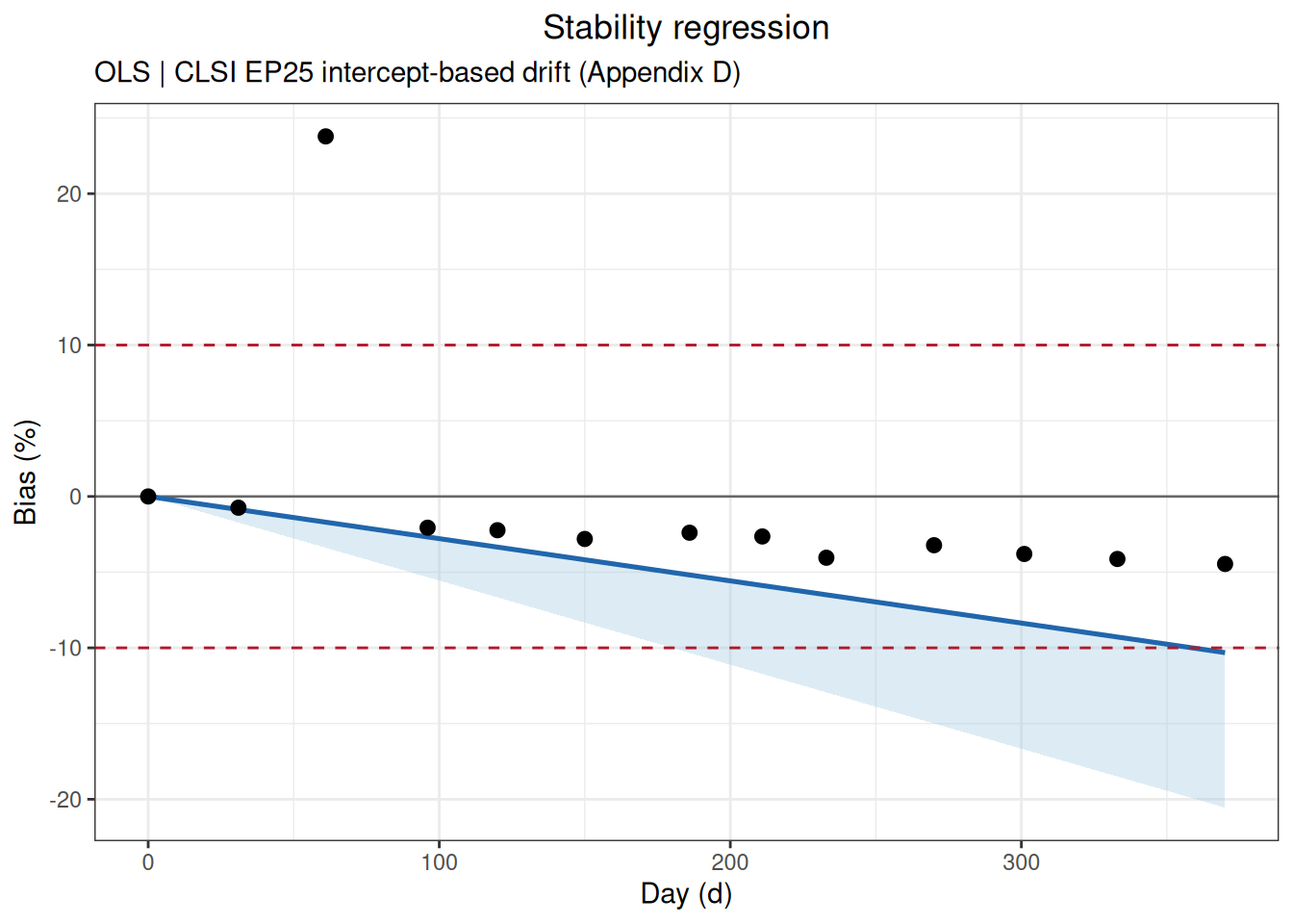

Cook 距离：

stability_regression() 已在返回对象中计算每个时间点的 Cook 距离，并将 Cook 距离大于 1 的观测记录在 diagnostics$influential 中：

代码

ep25_c5_cook_distance <- data.frame(
  Day = ep25_c5_data$Day,
  Cook_distance = unname(ep25_c5_with_result$diagnostics$cook_distance)
)
ep25_c5_cook_distance

   Day Cook_distance
1    0  1.172637e-01
2   31  7.185586e-02
3   61  1.078556e+00
4   96  2.477807e-02
5  120  1.448582e-02
6  150  9.639484e-03
7  186  2.404885e-03
8  211  1.263118e-03
9  233  4.142662e-03
10 270  1.404264e-06
11 301  3.051755e-04
12 333  3.335777e-03
13 370  1.752518e-02

代码

ep25_c5_influential <- ep25_c5_cook_distance[
  ep25_c5_cook_distance$Cook_distance > 1,
]
ep25_c5_influential

  Day Cook_distance
3  61      1.078556

与标准原文结果比较：

EP25 附录 C5：ivdtools 与标准原文结果对照
appendix	statistic	standard	ivdtools
EP25-A2 Appendix C5 / with_outlier	cook_distance_day_61	1.08	1.078556
EP25-A2 Appendix C5 / with_outlier	change_333	-9.28	-9.284424
EP25-A2 Appendix C5 / with_outlier	change_333_upper_CL	-18.50	-18.495388
EP25-A2 Appendix C5 / with_outlier	change_370	-10.32	-10.316027
EP25-A2 Appendix C5 / with_outlier	change_370_upper_CL	-20.55	-20.550431
EP25-A2 Appendix C5 / without_day_61	change_333	-3.68	-3.682110
EP25-A2 Appendix C5 / without_day_61	change_333_upper_CL	-4.38	-4.382553
EP25-A2 Appendix C5 / without_day_61	change_370	-4.09	-4.091233
EP25-A2 Appendix C5 / without_day_61	change_370_upper_CL	-4.87	-4.869504

4.1 主要函数

4.1.1 建立分析计划 stability_plan()

4.1.2 偏差分析 stability_bias()

4.1.3 不同保存条件比较的回归分析 stability_regression()

4.1.4 与首节点比较的回归分析 stability_regression()

4.1.5 预测达到限值的时间 stability_time()

4.1.6 阿伦纽斯（Arrhenius）加速稳定性分析 arrhenius()

4.1.7 MKT 计算 mkt()

4.1.8 多样本数据（长表）拆分

4.2 分析案例

4.2.1 CLSI EP25-A2 附录 B 阿伦纽斯加速稳定性

4.2.2 CLSI EP25-A2 附录 C1 试剂稳定性

4.2.3 CLSI EP25-A2 附录 C2.1 校准品稳定性（参考锚定实时研究）

4.2.4 CLSI EP25-A2 附录 C2.2 校准品稳定性（等时研究）

4.2.5 CLSI EP25-A2 附录 C3.1 控制品稳定性（参考锚定实时研究）

4.2.6 CLSI EP25-A2 附录 C3.2 控制品稳定性（等时研究）

4.2.7 CLSI EP25-A2 附录 C4 运输条件

4.2.8 CLSI EP25-A2 附录 C5 离群值评价

4.1.1 建立分析计划 `stability_plan()`

4.1.2 偏差分析 `stability_bias()`

4.1.3 不同保存条件比较的回归分析 `stability_regression()`

4.1.4 与首节点比较的回归分析 `stability_regression()`

4.1.5 预测达到限值的时间 `stability_time()`

4.1.6 阿伦纽斯（Arrhenius）加速稳定性分析 `arrhenius()`

4.1.7 MKT 计算 `mkt()`