14 线性分析

线性（linearity）评价测量系统在整个工作范围内，测得结果与被测物浓度（或目标量值）之间是否存在可接受的线性关系，通常采用稀释数据，按 CLSI EP06 分析偏差。本文统一使用专用的 linearity() 工作流完成水平汇总、权重、直线残差、允许偏离线性（ADL）和探索性多项式分析。

使用边界

EP06 第 2 版的核心是相对于预设允许偏离线性（ADL）评价直线残差，而不是以相关系数或“二次项不显著”单独证明线性。method="linear" 在水平均值上拟合；method="polynomial" 复现已被取代的 EP6-A 思路，应明确标为探索性。函数不替代样品配制、可交换性、端点覆盖、干扰和报告范围的专业判断。

分析流程：验证报告范围内的线性和允许偏离

%%{init: {"theme":"base","themeVariables":{"primaryColor":"#EAF2FB","primaryBorderColor":"#2780E3","primaryTextColor":"#212529","lineColor":"#6C757D","secondaryColor":"#EAF7E6","tertiaryColor":"#FFF4E8","fontSize":"13px"},"flowchart":{"nodeSpacing":18,"rankSpacing":24,"padding":6}}}%%

flowchart LR
    A["设计 LOW/HIGH<br/>与稀释水平"] --> B["linearity_replicates()<br/>linearity_panel()"]
    B --> C["重复测量长表"]
    C --> D["linearity()<br/>内部完成水平汇总与拟合"]
    D --> E["残差、区间<br/>与 ADL 比较"]
    E --> F["linearity_endpoints()<br/>核对报告端点"]
    F --> G["仅在验证范围内<br/>声明线性"]

    classDef input fill:#EAF2FB,stroke:#2780E3,color:#212529
    classDef process fill:#EAF7E6,stroke:#3FB618,color:#212529
    classDef output fill:#F4EEFB,stroke:#9954BB,color:#212529
    class A,C input
    class B,D,E,F process
    class G output

代码

library(ivdtools)
library(readr)

14.1 主要函数

函数	主要用途	关键输入或输出
`linearity_replicates()`	按精密度和 ADL 计算每水平重复数	`imprecision`、`adl`、 `family_error`
`linearity_panel()`	设计 HIGH/LOW 配制系列	`proportion_high`、`high`、`low`、 `total_volume`
`linearity_endpoints()`	计算 LOW/HIGH 实验室确认目标	LLoQ/ULoQ 与低高端 CV
`linearity()`	EP06 参数化线性分析	`method`、`weights`、`conf.level`、 `adl_*`
`plot()`	绘制重复结果、精密度、拟合、残差或模型差异	`type`

14.1.0.1 设计重复数与配制水平

代码

linearity_replicates(
  imprecision = 4,
  adl = 5,
  levels = 8,
  family_error = 0.10
)

  Type: relative
    Imprecision           : 4
    ADL                   : 5
    True deviation        : 0
    Effective ADL         : 5
    Level probability     : 0.98691628
    Z                     : 2.4814824
    Calculated replicates : 3.940963
    Replicates            : 4
    Recommend four        : FALSE

代码

linearity_panel(
  proportion_high = seq(0, 1, length.out = 6),
  high = 1000,
  low = 10,
  total_volume = 1
)

  Sample: S1
    Proportion high        : 0
    Proportion low         : 1
    Expected               : 10
    Relative concentration : 0.01
    Total volume           : 1
    High volume            : 0
    Low volume             : 1

  Sample: S2
    Proportion high        : 0.2
    Proportion low         : 0.8
    Expected               : 208
    Relative concentration : 0.208
    Total volume           : 1
    High volume            : 0.2
    Low volume             : 0.8

  Sample: S3
    Proportion high        : 0.4
    Proportion low         : 0.6
    Expected               : 406
    Relative concentration : 0.406
    Total volume           : 1
    High volume            : 0.4
    Low volume             : 0.6

  Sample: S4
    Proportion high        : 0.6
    Proportion low         : 0.4
    Expected               : 604
    Relative concentration : 0.604
    Total volume           : 1
    High volume            : 0.6
    Low volume             : 0.4

  Sample: S5
    Proportion high        : 0.8
    Proportion low         : 0.2
    Expected               : 802
    Relative concentration : 0.802
    Total volume           : 1
    High volume            : 0.8
    Low volume             : 0.2

  Sample: S6
    Proportion high        : 1
    Proportion low         : 0
    Expected               : 1000
    Relative concentration : 1
    Total volume           : 1
    High volume            : 1
    Low volume             : 0

代码

linearity_endpoints(
  lloq = 10, uloq = 1000,
  cv_high = 5, cv_at_lloq = 20, cv_at_k_lloq = 15
)

CLSI EP06-Ed2 target concentrations
  LOW target: 14.14116
  HIGH target: 924.0072

重复数函数只报告统计设计量；最终水平数和重复数还应满足研究方案、适用标准与样本资源约束；计算 LOW/HIGH 限制在实验室确认目标浓度使用，不适用于厂商的验证过程。

14.1.0.2 直线模型、区间与 ADL

下面直接使用每行一条重复测量的长表。sample 标识浓度水平，x 为预期值；同一 sample 内的 x 必须恒定。

代码

linearity_data <- read_csv("./data/014-线性分析/linearity-dilution.csv", show_col_types = FALSE)
linearity_data <- as.data.frame(linearity_data)

lin_ep06 <- linearity(
  linearity_data,
  sample = "conc",
  result = "signal",
  x = "conc",
  method = "linear",
  weights = "level_variance",
  conf.level = 0.95,
  multiplicity = "familywise",
  adl_rel = 5
)
lin_ep06

Linearity regression analysis

Analysis settings

Method: linear (EP06-Ed2)
Observations / levels: 24 / 8
Intercept: estimated
Weights: level_variance
Fit unit: level_mean

Model comparison

Degree: 1
Observations                : 8
Parameters                  : 2
Residual degrees of freedom : 6
RSS                         : 158.54622
Weighted RSS                : 7.7423768
SY.X                        : 5.1404639
Weighted SY.X               : 1.135956
R-squared                   : 0.99998216
Adjusted R-squared          : 0.99997918

Regression coefficients

     Estimate  Std. Error   t value   Pr(>|t|)    
a -0.12687310  0.39305554  -0.32279    0.75781    
b  0.99947673  0.00172361 579.87366 1.7753e-15 ***
---
Signif. codes:  0 '***' 0.001 '**' 0.01 '*' 0.05 '.' 0.1 ' ' 1

Sample fit information

Sample  Expected  Predicted  Observed mean      Weight  Observed SD  n
50            50    49.8470        49.2667  6.08108108     0.702377  3
100          100    99.8208       100.8000  3.29670330     0.953939  3
200          200   199.7685       202.6667  0.15133681     4.452340  3
400          400   399.6638       397.8333  0.05484127     7.396170  3
800          800   799.4545       798.8667  0.02848913    10.261741  3
1600        1600  1599.0359      1596.9000  0.01585959    13.753545  3
3200        3200  3198.1987      3207.8000  0.00684119    20.940869  3
6400        6400  6396.5242      6389.5667  0.00755775    19.923437  3

Sample bias information

Sample   Residual  Recovery bias  Residual (%)  Recovery bias (%)        ADL  Decision  
50      -0.580297      -0.733333    -1.1641563          -1.466667    2.49235  Within ADL
100      0.979200       0.800000     0.9809583           0.800000    4.99104  Within ADL
200      2.898194       2.666667     1.4507766           1.333333    9.98842  Within ADL
400     -1.830484      -2.166667    -0.4580060          -0.541667   19.98319  Within ADL
800     -0.587842      -1.133333    -0.0735304          -0.141667   39.97273  Within ADL
1600    -2.135890      -3.100000    -0.1335736          -0.193750   79.95179  Within ADL
3200     9.601346       7.800000     0.3002111           0.243750  159.90993  Within ADL
6400    -6.957514     -10.433333    -0.1087702          -0.163021  319.82621  Within ADL

Definitions

Residual = observed mean - predicted value.
Recovery bias = observed mean - expected value.
Recovery bias (%) = 100 * recovery bias / expected value.
Residual (%) denominator: predicted.
ADL decision metric = residual.

代码

plot(lin_ep06, type = "fit")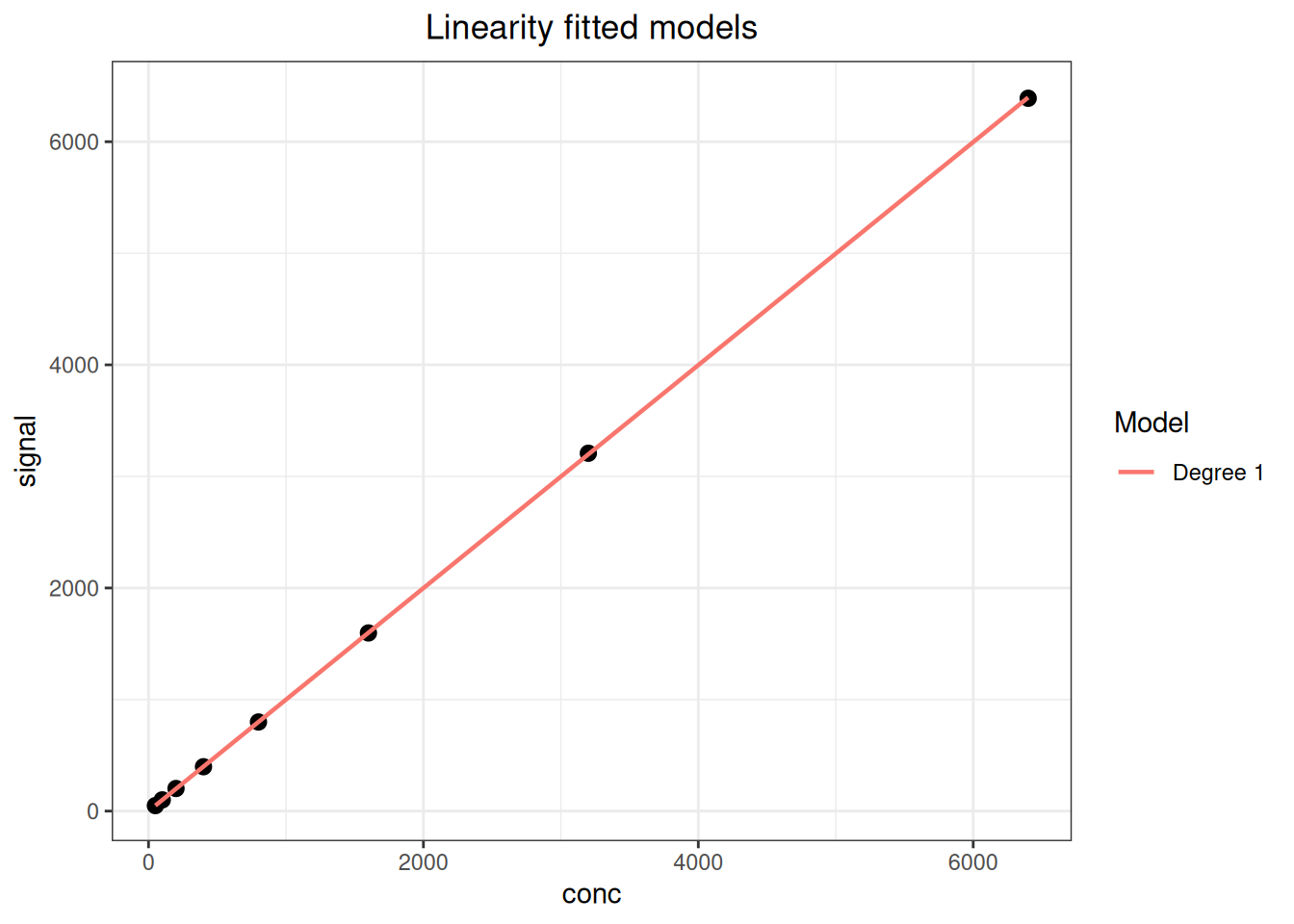

代码

plot(lin_ep06, type = "residual")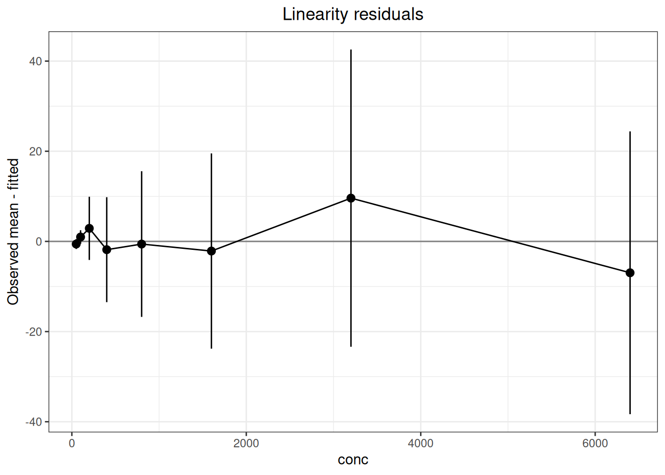

adl_exceeded 是实测线性偏离与调用者提供 ADL 的数值比较，不代表完整的产品合格结论。多项式模式用于复现旧版 EP6-A 思路，在 EP06-Ed2 语境下应标为探索性分析。

14.1.1 设计量、权重与允许偏离公式

代码

linearity_replicates(
  imprecision, adl, type = c("relative", "absolute"),
  level_probability = 0.99, levels = NULL, family_error = NULL,
  true_deviation = 0, min_replicates = 2
)
linearity_panel(proportion_high, high, low = 0,
                total_volume = NULL, sample = NULL)
linearity(
  data, sample, result, x, method = c("linear", "polynomial"),
  intercept = TRUE,
  weights = c("equal", "level_variance", "pooled", "precision_profile"),
  variance_group = NULL,
  conf.level = NULL, multiplicity = c("familywise", "none"),
  adl = NULL, adl_abs = NULL, adl_rel = NULL
)

若单水平中心覆盖概率为 \(P_L\)，重复性为 \(s\) 或 CV，预期真实偏离为 \(\delta_0\)，有效 ADL 为 \(A_{\mathrm{eff}}=A-\delta_0\)，重复数按

\[ n=\left\lceil\left(\frac{z_{(1+P_L)/2}s}{A_{\mathrm{eff}}}\right)^2\right\rceil \]

并受 min_replicates 限制。给出总族错误概率 \(\alpha_F\) 和 \(L\) 个水平时，\(P_L=(1-\alpha_F)^{1/L}\)。相对型输入统一使用百分数单位，例如 5 表示 5%。

HIGH/LOW 面板中，高样品比例为 \(p_h\) 时

\[ x_{\mathrm{expected}}=p_hx_H+(1-p_h)x_L. \]

linearity(method="linear") 先按样本汇总 \(\bar y_j,s_j,n_j\)，拟合 \(\bar y_j=\beta_0+\beta_1x_j+e_j\)。权重差异为：

`weights`	水平均值拟合权重	适用含义
`equal`	\(1\)	各水平等权
`level_variance`	\(n_j/s_j^2\)	使用各水平自身重复方差
`pooled`	\(n_j/\widehat\sigma_g^2\)	按 `variance_group` 明确指定的相邻水平组合并方差；不自动分组
`precision_profile`	\(1/\widehat\sigma_j^2\)	用 SD—均值轮廓预测方差

直线残差为 \(r_j=\bar y_j-\widehat y_j\)。adl_abs、adl_rel 或逐水平 adl 同时给出时，函数逐水平采用最大的允许值；相对 ADL 转为绝对量后比较

\[ |r_j|>ADL_j. \]

weights="pooled" 时，variance_group 必须指向原数据中的分组列；同一样本水平的分组值必须相同，各组在按 \(x\) 排序后必须连续且至少含两个水平。组内合并方差为

\[ \widehat\sigma_g^2= \frac{\sum_{j\in g}(n_j-1)s_j^2}{\sum_{j\in g}(n_j-1)}, \]

水平均值回归权重为 \(n_j/\widehat\sigma_g^2\)。percent_base 决定相对残差分母是直线预测值、\(x\) 还是观测均值。multiplicity="familywise" 把总体覆盖度换为逐水平覆盖度 \(C_L=C^{1/L}\)；"none" 则每个水平直接使用 \(C\)。

linearity_replicates() 返回设计重复数；linearity_panel() 返回配制水平表；linearity_endpoints() 返回低、高端目标；linearity() 返回含水平汇总、拟合、残差和 ADL 比较的分析对象；plot() 返回 ggplot 对象。

14.2 分析案例

14.2.1 示例一：系列稀释的线性偏差

稀释系列包含 8 个浓度水平、每水平 3 次重复，共 24 行：

代码

dilution <- read_csv("./data/014-线性分析/linearity-dilution.csv", show_col_types = FALSE)
dilution <- as.data.frame(dilution)
head(dilution, 6)

  conc replicate signal
1   50         1   48.6
2   50         2   49.2
3   50         3   50.0
4  100         1  101.3
5  100         2   99.7
6  100         3  101.4

linearity() 直接接收每行一条重复结果的长表，在函数内部按 sample 汇总均值、SD 和重复数，再拟合水平均值。这里用各水平等权重，并以预设的相对 ADL 评价直线残差：

代码

fit_lin <- linearity(
  dilution,
  sample = "conc",
  result = "signal",
  x = "conc",
  method = "linear",
  weights = "equal",
  conf.level = 0.95,
  multiplicity = "familywise",
  adl_rel = 5
)
print(fit_lin)

Linearity regression analysis

Analysis settings

Method: linear (EP06-Ed2)
Observations / levels: 24 / 8
Intercept: estimated
Weights: equal
Fit unit: level_mean

Model comparison

Degree: 1
Observations                : 8
Parameters                  : 2
Residual degrees of freedom : 6
RSS                         : 146.65863
Weighted RSS                : 146.65863
SY.X                        : 4.9439969
Weighted SY.X               : 4.9439969
R-squared                   : 0.99999571
Adjusted R-squared          : 0.999995

Regression coefficients

     Estimate  Std. Error    t value Pr(>|t|)    
a 0.975290473 2.205878722    0.44213  0.67388    
b 0.998893935 0.000844269 1183.14720  < 2e-16 ***
---
Signif. codes:  0 '***' 0.001 '**' 0.01 '*' 0.05 '.' 0.1 ' ' 1

Sample fit information

Sample  Expected  Predicted  Observed mean  Weight  Observed SD  n
50            50     50.920        49.2667       1     0.702377  3
100          100    100.865       100.8000       1     0.953939  3
200          200    200.754       202.6667       1     4.452340  3
400          400    400.533       397.8333       1     7.396170  3
800          800    800.090       798.8667       1    10.261741  3
1600        1600   1599.206      1596.9000       1    13.753545  3
3200        3200   3197.436      3207.8000       1    20.940869  3
6400        6400   6393.896      6389.5667       1    19.923437  3

Sample bias information

Sample   Residual  Recovery bias  Residual (%)  Recovery bias (%)        ADL  Decision  
50      -1.653321      -0.733333    -3.2468990          -1.466667    2.54600  Within ADL
100     -0.064684       0.800000    -0.0641295           0.800000    5.04323  Within ADL
200      1.912589       2.666667     0.9527025           1.333333   10.03770  Within ADL
400     -2.699531      -2.166667    -0.6739850          -0.541667   20.02664  Within ADL
800     -1.223772      -1.133333    -0.1529542          -0.141667   40.00452  Within ADL
1600    -2.305587      -3.100000    -0.1441708          -0.193750   79.96028  Within ADL
3200    10.364116       7.800000     0.3241384           0.243750  159.87179  Within ADL
6400    -4.329810     -10.433333    -0.0677179          -0.163021  319.69482  Within ADL

Definitions

Residual = observed mean - predicted value.
Recovery bias = observed mean - expected value.
Recovery bias (%) = 100 * recovery bias / expected value.
Residual (%) denominator: predicted.
ADL decision metric = residual.

ADL 是否超限只能按方案预先规定的限值解释。 weights 可选等权、各水平自身方差、预设分组的合并方差或精密度轮廓；选择应与试验设计和异方差结构一致。

代码

plot(fit_lin, type = "fit")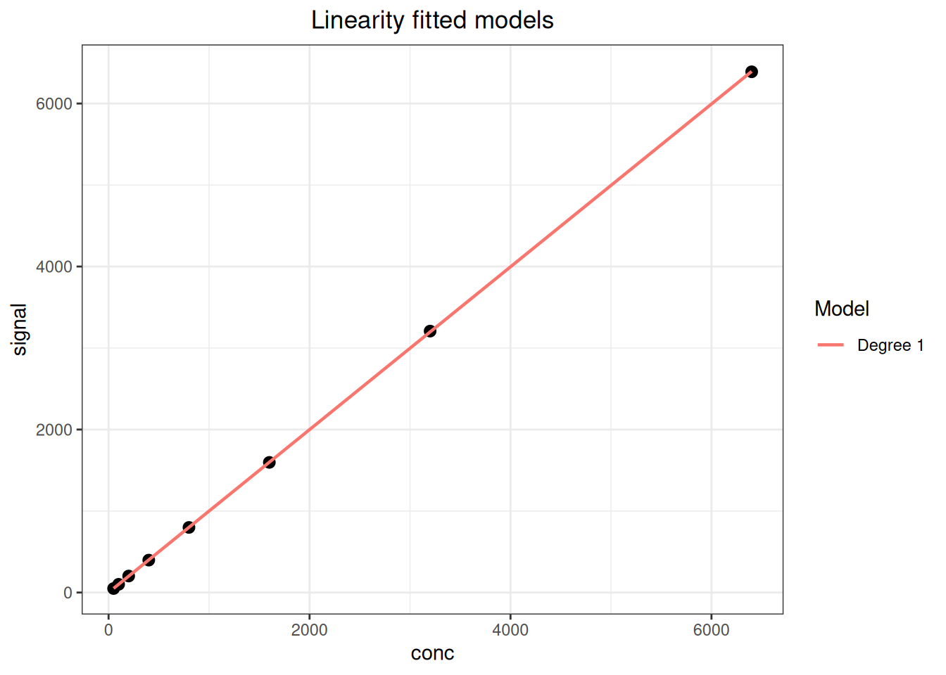

代码

plot(fit_lin, type = "residual")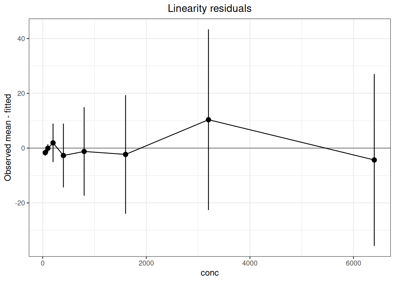

14.2.2 示例二：对半稀释的多项式分析

数据为 5 个浓度水平 × 3 复孔：

代码

poly_data <- read_csv("./data/014-线性分析/linearity-polynomial.csv", show_col_types = FALSE)
poly_data <- as.data.frame(poly_data)
head(poly_data, 6)

    conc replicate signal
1  75.00         1   75.0
2  75.00         2   75.0
3  75.00         3   74.4
4 483.75         1  454.1
5 483.75         2  455.3
6 483.75         3  456.0

代码

fit_poly <- linearity(
  poly_data,
  sample = "conc",
  result = "signal",
  x = "conc",
  method = "polynomial",
  weights = "level_variance",
  max_degree = 3,
  poly_alpha = 0.05,
  percent_base = "predicted"
)
print(fit_poly)

Linearity regression analysis

Analysis settings

Method: polynomial (EP6-A, exploratory)
Observations / levels: 15 / 5
Intercept: estimated
Weights: level_variance
Fit unit: observation
Selected degree: 3

Model comparison

Degree: 1
Observations                : 15
Parameters                  : 2
Residual degrees of freedom : 13
RSS                         : 52631.917
Weighted RSS                : 550.93015
SY.X                        : 63.62868
Weighted SY.X               : 6.5099341
R-squared                   : 0.99902344
Adjusted R-squared          : 0.99894832

Degree: 2
Observations                : 15
Parameters                  : 3
Residual degrees of freedom : 12
RSS                         : 10241.163
Weighted RSS                : 30.175825
SY.X                        : 29.213529
Weighted SY.X               : 1.5857655
R-squared                   : 0.99994651
Adjusted R-squared          : 0.9999376

Degree: 3
Observations                : 15
Parameters                  : 4
Residual degrees of freedom : 11
RSS                         : 4360.5146
Weighted RSS                : 15.881083
SY.X                        : 19.910058
Weighted SY.X               : 1.2015552
R-squared                   : 0.99997185
Adjusted R-squared          : 0.99996417
Selected                    : Yes

Regression coefficients (degree 1)

    Estimate Std. Error   t value Pr(>|t|)    
a 3.26682147 1.60149874   2.03985 0.062224 .  
b 0.94635339 0.00820623 115.32135  < 2e-16 ***
---
Signif. codes:  0 '***' 0.001 '**' 0.01 '*' 0.05 '.' 0.1 ' ' 1

Regression coefficients (degree 2)

     Estimate  Std. Error  t value   Pr(>|t|)    
a 7.07723e+00 4.71485e-01  15.0105 3.8555e-09 ***
b 8.98365e-01 3.88796e-03 231.0636 < 2.22e-16 ***
c 5.87581e-05 4.08310e-06  14.3905 6.2393e-09 ***
---
Signif. codes:  0 '***' 0.001 '**' 0.01 '*' 0.05 '.' 0.1 ' ' 1

Regression coefficients (degree 3, selected)

      Estimate   Std. Error  t value   Pr(>|t|)    
a  1.08167e+01  1.24094e+00  8.71655 2.8637e-06 ***
b  8.38991e-01  1.90976e-02 43.93179 1.0374e-13 ***
c  1.93013e-04  4.27784e-05  4.51193  0.0008837 ***
d -5.97186e-08  1.89786e-08 -3.14662  0.0092980 ** 
---
Signif. codes:  0 '***' 0.001 '**' 0.01 '*' 0.05 '.' 0.1 ' ' 1

Sample fit information

Sample   Expected  Predicted  Observed mean      Weight  Observed SD  n
75          75.00    74.8015         74.800  8.33333333     0.346410  3
483.75     483.75   455.0861        455.133  1.08303249     0.960902  3
892.5      892.50   870.9067        865.967  0.01552474     8.025792  3
1301.25   1301.25  1297.7933       1328.467  0.00166688    24.493332  3
1710      1710.00  1711.2760       1710.433  0.01516914     8.119319  3

Sample bias information

Sample      Residual  Recovery bias  Residual (%)  Recovery bias (%)         DL  ADL  Decision    
75       -0.00153386      -0.200000   -0.00206599         -0.2666667   0.558208   NA  Not assessed
483.75    0.04720887     -28.616667    0.01023909         -5.9155900  -5.979149   NA  Not assessed
892.5    -4.94005897     -26.533333   -0.58263161         -2.9729225  23.019504   NA  Not assessed
1301.25  30.67332481      27.216667    2.48425504          2.0915786  63.084173   NA  Not assessed
1710     -0.84264426       0.433333   -0.05196596          0.0253411  89.744861   NA  Not assessed

Definitions

Residual = observed mean - predicted value.
Recovery bias = observed mean - expected value.
Recovery bias (%) = 100 * recovery bias / expected value.
Residual (%) denominator: predicted.
ADL decision metric = deviation from linearity (DL).

Warnings / interpretation notes

1 duplicate sample/result/x row(s) were retained.

Polynomial regression follows superseded EP6-A and is exploratory under EP06-Ed2.

代码

plot(fit_poly, type = "fit")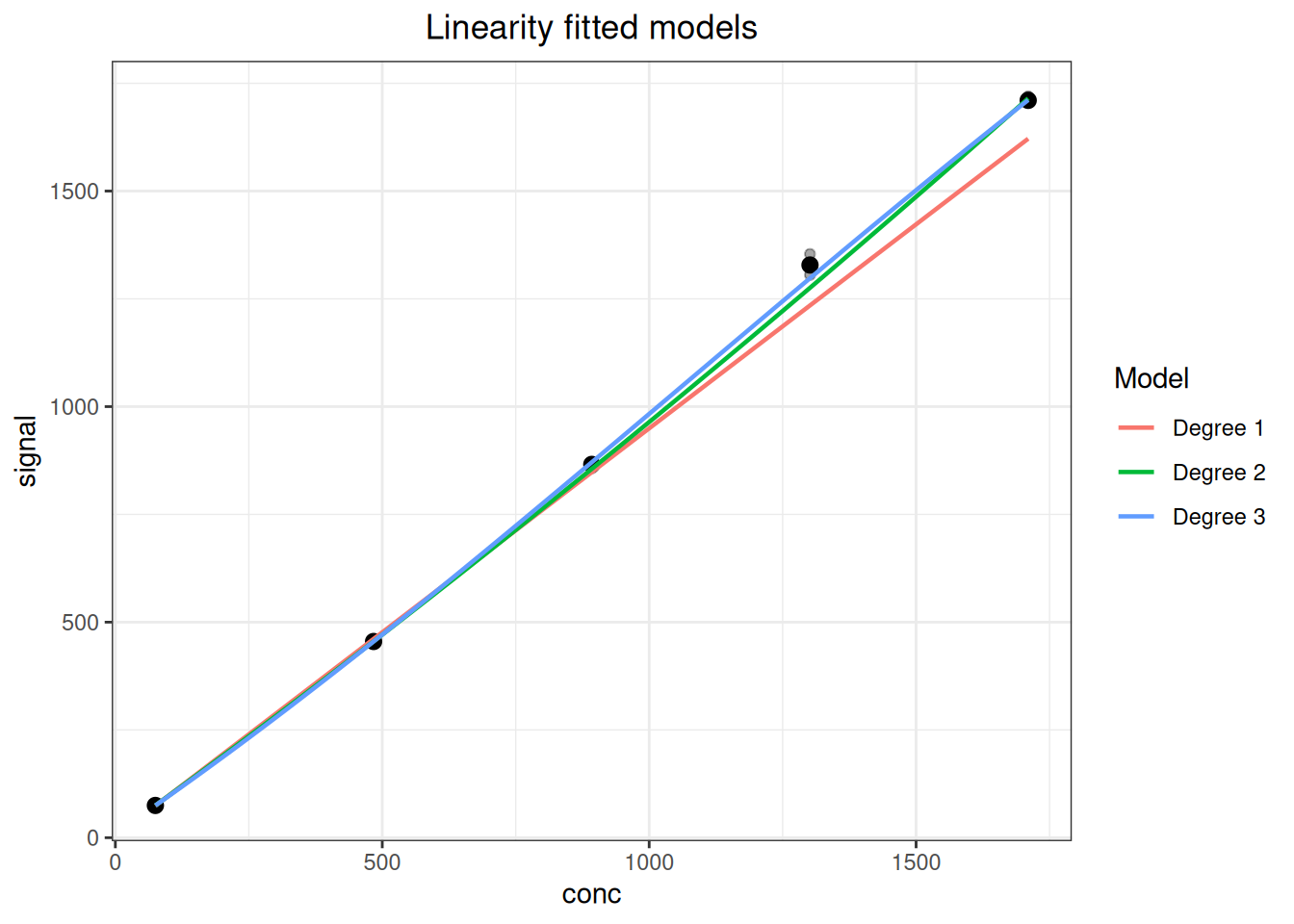

代码

plot(fit_poly, type = "difference")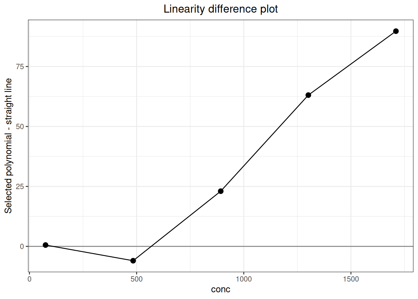

14.2.3 标准案例：CLSI EP06 第 2 版附录 G 两重复研究

附录 G 使用 HIGH 与空白按 0.1～1.0 相对浓度配制 10 个水平，每水平测量 2 次。预设线性区间为 55～500 U/L，允许偏离线性为 ±10%。标准因每水平仅有 2 次重复，将相邻水平的方差分成三组进行合并，再以 \(2/\overline{s^2}\) 作为无截距 WLS 权重。分组列已按标准表 G3 直接写入 CSV，预期浓度也已根据 HIGH 浓度和配制比例写入。

代码

ep06_g <- as.data.frame(read_csv(
  "./data/014-线性分析/std-ep06-appendix-g.csv",
  show_col_types = FALSE
))

代码

ep06_g_ivd <- linearity(
  ep06_g, sample = "level", result = "result", x = "expected",
  method = "linear", intercept = FALSE,
  weights = "pooled", variance_group = "variance_group"
)

EP06 第 2 版附录 G：ivdtools 与标准原文结果对照
标准位置	统计量	标准结果	ivdtools结果
EP06 Ed2 Appendix G	WLS_slope	1.0677	1.0677
EP06 Ed2 Appendix G	max_abs_deviation_percent	9.3000	9.2644

variance_group 将 10 个水平明确分成 1–3、4–7、8–10 三组。分组由用户根据重复性SD—浓度图和预先规定的方案提供，函数不自动选择最有利的分组。

14.2.4 标准案例：CLSI EP06 第 2 版附录 H 双面板研究

附录 H 用 HIGH1 和 HIGH2 分别与空白配制两个 10 水平面板，每水平测量 5 次，共 100 条结果。HIGH1 覆盖高端，HIGH2 覆盖低端；合并后覆盖案例预设的 20～1000 U/L 区间。每水平权重为 \(5/s^2\)，拟合无截距 WLS 直线。CSV 已包含由面板、水平和配制比例确定的sample_id 与expected，读取后可直接进入分析。

代码

ep06_h <- as.data.frame(read_csv(
  "./data/014-线性分析/std-ep06-appendix-h.csv",
  show_col_types = FALSE
))

代码

ep06_h_fit <- function(z) {
  fit <- linearity(
    z, sample = "sample_id", result = "result", x = "expected",
    method = "linear", intercept = FALSE, weights = "level_variance"
  )
  data.frame(
    slope = fit$coefficients$estimate,
    max_abs_deviation_percent = max(abs(fit$level_summary$percent_residual_linear))
  )
}
ep06_h_combined <- ep06_h_fit(ep06_h)
ep06_h_separate <- do.call(rbind, lapply(
  split(ep06_h, ep06_h$panel), ep06_h_fit
))

EP06 第 2 版附录 H：ivdtools 与标准原文结果对照
标准位置	统计量	标准结果	ivdtools结果
EP06 Ed2 Appendix H	combined WLS slope	0.9686	0.9686
EP06 Ed2 Appendix H	combined maximum deviation (%)	14.5000	14.4759
EP06 Ed2 Appendix H	HIGH1 WLS slope	0.9496	0.9496
EP06 Ed2 Appendix H	HIGH1 maximum deviation (%)	12.8000	12.7612
EP06 Ed2 Appendix H	HIGH2 WLS slope	1.0013	1.0013
EP06 Ed2 Appendix H	HIGH2 maximum deviation (%)	9.2000	9.2134

三种分析的最大偏离均未超过案例预设 ±15%，但两个部分面板的重叠、范围覆盖和权重结构是这一结论成立的前提。

14.2.5 标准案例：CLSI EP06 第 2 版附录 I 赋值样品

附录 I 给出 9 个加标样品的真值、10 次测量均值和 SD，但不公布 90 条单次测量结果。因此本例保留标准公布的汇总粒度，不从均值和 SD 反向生成伪原始数据。权重为 \(10/s^2\)，拟合无截距 WLS 直线，预设允许偏离为 ±2%。

代码

ep06_i <- as.data.frame(read_csv(
  "./data/014-线性分析/std-ep06-appendix-i-summary.csv",
  show_col_types = FALSE
))
ep06_i$weight <- ep06_i$n / ep06_i$sd^2
ep06_i_ivd <- linearity(
  ep06_i, sample = "sample", result = "measured_mean", x = "true_value",
  method = "linear", intercept = FALSE, weights = ep06_i$weight
)

EP06 第 2 版附录 I：ivdtools 与标准原文结果对照
标准位置	统计量	标准结果	ivdtools结果
EP06 Ed2 Appendix I	WLS_slope	1.0045	1.0045
EP06 Ed2 Appendix I	max_abs_deviation_percent	1.7000	1.7212

复算的最大绝对偏离位于案例预设 ±2% 内。回收偏差与线性偏离回答不同问题：前者相对真值，后者相对最佳拟合直线，不能互相替代。

14.2.6 标准案例：WS/T 408—2024 五水平线性验证

附录 A.4 的 HDL-C 案例包含 5 个水平、每水平 3 次测量。标准关注直线回归剩余标准差 \(s_{y|x}\)、批内标准差 \(s_{WR}\)、二者的 F 比值及非线性标准差 \(s_{NL}\)。

代码

wst408_linearity <- read_csv(
  "./data/014-线性分析/std-wst408-linearity.csv",
  show_col_types = FALSE
)

wst408_linearity_ivd <- linearity(
  as.data.frame(wst408_linearity), sample = "level", result = "measured",
  x = "expected", method = "linear", conf.level = 0.95
)

WS/T 408 附录 A.4：ivdtools 与标准原文结果对照
标准位置	统计量	标准结果	ivdtools结果
WS/T 408 Appendix A.4	s_yx	0.0318	0.03277
WS/T 408 Appendix A.4	s_WR	0.0186	NA
WS/T 408 Appendix A.4	F	2.9130	NA
WS/T 408 Appendix A.4	s_NL	0.0258	NA

linearity() 按 5 个水平均值拟合直线，输出 \(s_{y|x}\approx0.0328\)；标准配套表为 0.0318。标准所需的 \(s_{WR}\)、F 和 \(s_{NL}\) 不是当前对象的公开结果，表中以 NA 明示未实现。

14.2.7 标准案例：YY/T 1789.4—2022 附录 A 线性样本 1

附录 A.5 给出 AFP 线性样本 1 的 14 个稀释水平、每水平 4 次结果。标准先用一至三阶多项式的高阶项显著性选择模型，再以最终直线的逐水平相对偏倚和 ±10% 允许误差判断测量区间。

代码

yyt1789_4 <- read.csv(
  "./data/014-线性分析/std-yyt1789-4-appendix-a-sample1.csv"
)
yyt1789_4_linear_p <- linearity(
  yyt1789_4, sample = "level", result = "result", x = "dilution",
  method = "polynomial", weights = "equal", adl_rel = 10
)
yyt1789_4_linear <- linearity(
  yyt1789_4, sample = "level", result = "result", x = "dilution",
  method = "linear", weights = "equal", adl_rel = 10
)

YY/T 1789.4—2022 附录 A.5：最终直线和相对偏倚对照
标准位置	统计量	标准结果	ivdtools结果
YY/T 1789.4 Appendix A.5 / level 1	final-line prediction	4.28	4.284
YY/T 1789.4 Appendix A.5 / level 1	relative bias (%)	6.07	5.974
YY/T 1789.4 Appendix A.5 / level 2	final-line prediction	19.40	19.401
YY/T 1789.4 Appendix A.5 / level 2	relative bias (%)	5.05	5.046
YY/T 1789.4 Appendix A.5 / level 3	final-line prediction	34.52	34.518
YY/T 1789.4 Appendix A.5 / level 3	relative bias (%)	4.46	4.453
YY/T 1789.4 Appendix A.5 / level 4	final-line prediction	64.75	64.752
YY/T 1789.4 Appendix A.5 / level 4	relative bias (%)	-3.69	-3.697
YY/T 1789.4 Appendix A.5 / level 5	final-line prediction	125.22	125.219
YY/T 1789.4 Appendix A.5 / level 5	relative bias (%)	7.25	7.250
YY/T 1789.4 Appendix A.5 / level 6	final-line prediction	246.16	246.154
YY/T 1789.4 Appendix A.5 / level 6	relative bias (%)	0.47	0.467
YY/T 1789.4 Appendix A.5 / level 7	final-line prediction	367.10	367.089
YY/T 1789.4 Appendix A.5 / level 7	relative bias (%)	3.77	3.773
YY/T 1789.4 Appendix A.5 / level 8	final-line prediction	488.04	488.025
YY/T 1789.4 Appendix A.5 / level 8	relative bias (%)	-4.04	-4.043
YY/T 1789.4 Appendix A.5 / level 9	final-line prediction	608.98	608.960
YY/T 1789.4 Appendix A.5 / level 9	relative bias (%)	-3.05	-3.051
YY/T 1789.4 Appendix A.5 / level 10	final-line prediction	729.92	729.895
YY/T 1789.4 Appendix A.5 / level 10	relative bias (%)	3.59	3.598
YY/T 1789.4 Appendix A.5 / level 11	final-line prediction	850.86	850.830
YY/T 1789.4 Appendix A.5 / level 11	relative bias (%)	-3.99	-3.990
YY/T 1789.4 Appendix A.5 / level 12	final-line prediction	971.80	971.765
YY/T 1789.4 Appendix A.5 / level 12	relative bias (%)	2.60	2.607
YY/T 1789.4 Appendix A.5 / level 13	final-line prediction	1092.74	1092.700
YY/T 1789.4 Appendix A.5 / level 13	relative bias (%)	-3.20	-3.198
YY/T 1789.4 Appendix A.5 / level 14	final-line prediction	1213.68	1213.635
YY/T 1789.4 Appendix A.5 / level 14	relative bias (%)	2.56	2.566

模型选择步骤并不完全等价：标准对水平均值拟合多项式并报告回归标准误， linearity(method="polynomial") 当前对逐次观测拟合，且将该模式标为旧 EP6-A 探索流程；两者自由度和回归标准误不同。因此本例只把包内 method="linear" 的最终直线称为复现，不把包的多项式选择结果冒充 YY/T 1789.4 的高阶项检验。

标准附录 A.3 的 ADL-PctBnd 临界表还把回归不精密度、水平数和重复数共同换算为临界值；adl_rel=10 是逐水平数值限，未实现 PctBnd 查表规则。这两个“ADL”名称相近但算法不同，本章报告时必须注明采用哪一种。