12 ROC 曲线与多元回归

本文在单标记物 ROC 的基础上，演示用多个标记物拟合二项 Logistic 回归、计算联合预测概率、绘制训练集 ROC，并对新样本预测。联合模型需要同时评价区分度、校准、临床效用和可推广性；AUC 增加只是其中一个方面。

使用边界

mlr() 拟合的是给定变量的未惩罚、主效应 Logistic 回归。当前 ivdtools 不进行变量筛选、非线性项自动构造、交互作用搜索、缺失值插补、共线性诊断、内部验证、校准评价、决策曲线、外部验证或模型更新。

mlr() 报告的联合 AUC 来自拟合模型所用的同一批数据，属于表观性能；其 Hanley–McNeil 区间也没有校正模型拟合和变量选择带来的乐观偏倚。predict() 给出的区间是模型系数不确定性所对应的平均预测概率置信区间，不是未来个体结局的预测区间。

多标记物工作流为：

%%{init: {"theme":"base","themeVariables":{"primaryColor":"#EAF2FB","primaryBorderColor":"#2780E3","primaryTextColor":"#212529","lineColor":"#6C757D","secondaryColor":"#EAF7E6","tertiaryColor":"#FFF4E8","fontSize":"13px"},"flowchart":{"nodeSpacing":18,"rankSpacing":24,"padding":6}}}%%

flowchart LR
    A["共同病例<br/>多个定量标记物"] --> B["roc() → auc()<br/>单标记物基线"]
    B --> C["mlr()<br/>Logistic 联合模型"]
    B --> G["auc_compare()<br/>配对 AUC 比较"]
    C --> G
    C --> D["系数与训练集 AUC"]
    C --> E["predict()<br/>新样本概率"]
    D --> F["独立验证<br/>区分度、校准、效用"]
    E --> F

    classDef input fill:#EAF2FB,stroke:#2780E3,color:#212529
    classDef process fill:#EAF7E6,stroke:#3FB618,color:#212529
    classDef output fill:#F4EEFB,stroke:#9954BB,color:#212529
    class A input
    class B,C,G,D,E process
    class F output

代码

library(ivdtools)
library(readr)

12.1 主要函数

函数	主要用途	主要结果
`roc()`	用多个标记物建立共同完整病例对象	标记物值、参考状态和单标记物方向
`auc()`	建立单标记物性能基线	每列 AUC、Hanley–McNeil SE 和 CI
`mlr()`	拟合一个命名的多元 Logistic 模型	模型、系数、预测概率及训练集 ROC/AUC
`auc_compare()`	比较同一批受试者的两条 ROC 曲线	AUC 差、SE、CI、z 和 P 值
`predict()`	用已保存模型预测训练数据或新数据	概率、SE、CI 和固定 0.5 分类
`plot()`	叠加原始标记物和联合模型 ROC	`ggplot` 图形
`summary()`	汇总所有已执行的分析	单标记物及全部命名模型结果

roc()、auc() 的完整参数、方向、AUC 和区间公式见上一章。本章重点说明联合模型接口。

12.1.1 多元 Logistic 回归 `mlr()`

代码

mlr(x, cols = NULL, name = NULL, ...)

参数	说明
`x`	已执行 `auc()` 的 `roc` 对象。
`cols`	进入模型的标记物列；`NULL` 使用对象中的全部标记物。
`name`	唯一模型名；省略时依次生成 `MLR01`、`MLR02` 等。
`...`	传给 `stats::glm()` 的其他参数，例如控制选项；模型公式和二项分布由函数固定。

令 \(Y_i\in\{0,1\}\)，选择 \(p\) 个标记物后，当前函数建立

\[ \eta_i=\beta_0+\sum_{j=1}^{p}\beta_jx_{ij}, \qquad \pi_i=P(Y_i=1\mid\mathbf x_i) =\frac{\exp(\eta_i)}{1+\exp(\eta_i)}. \]

系数通过二项分布最大似然估计。对其他变量不变的条件下，\(x_j\) 每增加一个原始单位，阳性优势乘以

\[ \operatorname{OR}_j=\exp(\beta_j). \]

这不是风险比，也不表示因果效应。若变量单位很小或很大，应在建模前按照预设方案缩放，以便系数具有可解释单位。

函数公式固定为 reference_binary ~ x1 + x2 + ...，不会自动加入平方项、样条或交互项。roc() 已经按全部初始 cols 建立共同完整病例，因此 mlr(cols=...) 的子模型仍使用同一分析集。这有利于比较嵌套标记物组合，但不等于完成缺失数据处理。

拟合后用同一批病例的 \(\widehat\pi_i\) 建经验 ROC，方向固定为 geq，即预测概率越大越倾向阳性。联合 AUC 的 SE 和 95% CI 继续使用上一章的 Hanley–McNeil 单曲线公式。

每个模型保存在 mlr_results[[name]]，主要字段为：

字段	含义
`formula`、`cols`	实际公式和预测变量
`fit`、`fit_summary`	`glm` 对象及其摘要
`predicted`	训练集拟合概率
`auc`、`auc_se`、`ci_lower`、`ci_upper`	训练集 AUC 及近似区间
`roc_curve`	训练概率的完整 cutoff 指标表

返回更新后的 roc 对象；新模型保存在 mlr_results[[name]]。

AUC 增加不等于模型已经得到验证

单标记物和联合模型的 ROC 来自同一受试者，二者相关，应使用 auc_compare() 作配对比较。但是，训练集联合概率由同一批结局数据拟合，EP24 和 DeLong 都把输入评分当作既定值，不会校正模型拟合、变量选择或过拟合造成的乐观偏倚。因此配对 P 值不能代替内部验证、独立验证、校准和临床净获益评价。

12.1.2 配对 AUC 比较 `auc_compare()`

代码

auc_compare(
  x,
  curves,
  method = c("ep24", "delong"),
  conf.level = 0.95,
  rating_method = c("pearson", "kendall"),
  name = NULL
)

参数	说明
`x`	已完成相应 `auc()` 或 `mlr()` 分析的同一个 `roc` 对象。
`curves`	恰好两个曲线名称，可以是原始标记物、命名 MLR，或两者各一个；差值方向为第一个减第二个。
`method`	默认 `"ep24"`，使用 EP24-A2 Hanley–McNeil 配对近似；`"delong"` 使用非参数配对协方差。
`conf.level`	AUC 差值区间的置信水平。
`rating_method`	EP24 组内评分相关方法；连续实验室结果默认 Pearson，有序等级可选 Kendall。DeLong 不使用该参数。
`name`	可选结果名称；省略时由两条曲线名称和方法自动生成。

函数只接受同一个 roc 对象中的曲线，从而保证阳性、阴性状态和完整病例完全配对。结果保存在 auc_comparisons[[name]]，包含两条 AUC、各自 SE、差值、差值 SE、置信区间、z、P 值及方法专用的相关或协方差信息。summary() 会打印全部已保存比较。

EP24 方法先分别计算阳性组和阴性组内两项评分的相关系数，再取平均，并结合平均 AUC 对 EP24-A2 表 5 作线性插值，得到两个 AUC 估计量之间的相关系数。若坐标超出标准表范围，函数使用最近边界并在结果与控制台中明确标记。DeLong 方法则从阳性和阴性的配对秩贡献直接估计两条 AUC 的协方差，不使用 EP24 查表近似。

12.1.3 概率预测 `predict()`

代码

predict(
  object,
  mlr = NULL,
  newdata = NULL,
  column_map = NULL
)

参数	说明
`object`	至少含一个 `mlr()` 结果的 `roc` 对象。
`mlr`	模型名；对象只有一个模型时可省略，多个模型时必须指定。
`newdata`	新数据框；`NULL` 时返回共同完整训练数据的拟合结果。
`column_map`	命名字符向量，名称是新数据列，值是训练模型列，例如 `c(new_x1="x1")`。

设新样本设计向量为 \(\mathbf x_0=(1,x_{01},\ldots,x_{0p})^\mathsf T\)，链接尺度预测及其标准误为

\[ \widehat\eta_0=\mathbf x_0^\mathsf T\widehat{\boldsymbol\beta}, \qquad \operatorname{SE}(\widehat\eta_0) =\sqrt{\mathbf x_0^\mathsf T \widehat{\operatorname{Cov}}(\widehat{\boldsymbol\beta})\mathbf x_0}. \]

函数先在 logit 尺度建立

\[ \widehat\eta_0\pm z_{0.975}\operatorname{SE}(\widehat\eta_0), \]

再用 \(\operatorname{logit}^{-1}\) 转回概率尺度得到 ci_lower 和 ci_upper。概率尺度的 pred_se 使用 Delta 法：

\[ \operatorname{SE}(\widehat\pi_0) \approx \operatorname{SE}(\widehat\eta_0) \widehat\pi_0(1-\widehat\pi_0). \]

pred_class 固定为 \(I(\widehat\pi_0\ge0.5)\)，当前接口不能改成其他概率阈值。若研究方案使用不同决策阈值，应从 pred_prob 另行按预设规则分类并明确记录。

返回含输入行标识、pred_prob、pred_se、ci_lower、ci_upper 和 pred_class 的数据框。

12.1.4 ROC 绘图和汇总

plot() 不可见地返回 ggplot 对象；summary() 打印并不可见地返回输入的 roc 对象。

代码

plot(x, curves = NULL, cutpoint = NULL,
     type = c("roc", "cutoff"))
summary(x)

curves 与 auc_compare() 使用同一个曲线命名空间：既可以是原始标记物名称，也可以是 MLR 模型名称。plot(x, curves="all") 绘制全部原始标记物和已保存模型；plot(x, curves=c("x1", "combined")) 可混合选择，单独指定 "combined" 则只画该模型。curves=NULL 保持默认只画全部原始标记物。type="cutoff" 只支持在 curves 中指定一个原始标记物，暂不支持多元模型概率的 cutoff 图。cutpoint 只标注所选原始标记物。summary() 打印全部已保存模型和 auc_compare() 比较结果。

12.2 分析案例

12.2.1 教学数据：两个标记物联合模型

代码

mlr_dat <- as.data.frame(read_csv(
  "./data/012-ROC曲线与多元回归/roc-multimarker.csv",
  show_col_types = FALSE
))
head(mlr_dat)

  sid ref        x1        x2
1   1   0  5.510540  8.298655
2   2   0  3.188811 12.942968
3   3   0  8.126533 12.351778
4   4   0  6.159571 16.105370
5   5   0 11.118763 11.867919
6   6   0  2.736035 19.585368

先在同一共同病例集上计算两个原始标记物的 AUC：

代码

mlr_fit <- roc(
  mlr_dat, cols = c("x1", "x2"),
  reference = "ref", id = "sid"
)
mlr_fit <- auc(mlr_fit)


AUC Table
  Column               AUC          95% CI  Direction
  ------------------------------------------------------------ 
  x1                0.9219  [0.8712, 0.9727]       geq
  x2                0.8322  [0.7587, 0.9057]       geq

代码

mlr_fit


ROC Analysis
  Data class:        data.frame
  Total rows:        120
  Complete cases:    120
  Reference:         ref (binary)
  Reference coding:  binary (0/1)
  Positive / Neg:    60 / 60
  Evaluation cols:   2  (x1, x2)
  Duplicate IDs:     none

Analysis slots:
    [ ] Describe
    [x] AUC
    [ ] Paired AUC comparison
    [ ] Cutoff
    [ ] MLR

x1 和 x2 的 AUC 分别为 0.9219 和 0.8322；两者方向均为 geq。随后拟合预先指定的双标记物主效应模型：

代码

mlr_fit <- mlr(
  mlr_fit, cols = c("x1", "x2"), name = "combined"
)


Multivariate Logistic Regression (combined)
  -------------------------------------------------- 
  Formula: reference_binary ~ x1 + x2
  n = 120  (positive = 60, negative = 60)
  AUC = 0.9642  [0.9298, 0.9985]

  Coefficients:
                   Estimate Std. Error   z value     Pr(>|z|) 
    (Intercept) -13.6586717  2.7569949 -4.954188 7.263286e-07 
    x1            0.7638502  0.1549103  4.930919 8.184356e-07 
    x2            0.3949617  0.1064673  3.709700 2.075049e-04 

  * Note: AUC is evaluated on the same data used for fitting;
    the estimate may be optimistic.

拟合方程为

\[ \operatorname{logit}(\widehat\pi) =-13.6587+0.76385x_1+0.39496x_2. \]

在另一个标记物不变时，x1 和 x2 每增加一个原始单位的调整优势比分别约为 \(\exp(0.76385)=2.146\) 和 \(\exp(0.39496)=1.484\)。截距的指数通常没有实际意义，因为 \(x_1=x_2=0\) 可能不在数据范围内。

联合模型训练集 AUC 为 0.9642，95% CI 为 0.9298～0.9985。进一步把联合模型分别与两个原始标记物作 EP24 配对比较：

代码

mlr_fit <- auc_compare(
  mlr_fit, curves = c("combined", "x1"), method = "ep24"
)


Paired AUC Comparison
  Curves: combined - x1
  Method: EP24-A2 Hanley-McNeil paired approximation
  Subjects: 120 (positive = 60, negative = 60)
  AUC combined: 0.964167
  AUC x1: 0.921944
  Difference: 0.042222
  SE difference: 0.022111
  95.0% CI: [-0.001115, 0.085559]
  z = 1.909555
  p-value: 0.0561906
  Mean within-group rating correlation: 0.660442
  EP24 area correlation: 0.538934
  Note: fitted training probabilities are treated as fixed scores;
        model optimism and fitting uncertainty are not corrected.

代码

mlr_fit <- auc_compare(
  mlr_fit, curves = c("combined", "x2"), method = "ep24"
)


Paired AUC Comparison
  Curves: combined - x2
  Method: EP24-A2 Hanley-McNeil paired approximation
  Subjects: 120 (positive = 60, negative = 60)
  AUC combined: 0.964167
  AUC x2: 0.832222
  Difference: 0.131944
  SE difference: 0.035277
  95.0% CI: [0.062803, 0.201085]
  z = 3.740275
  p-value: 0.000183819
  Mean within-group rating correlation: 0.445998
  EP24 area correlation: 0.357226
  Note: fitted training probabilities are treated as fixed scores;
        model optimism and fitting uncertainty are not corrected.

联合训练模型与单标记物的配对 AUC 比较
比较	AUC差	SE	CI下限	CI上限	z	P值
combined - x1	0.04222	0.02211	-0.00111	0.08556	1.90955	0.05619
combined - x2	0.13194	0.03528	0.06280	0.20109	3.74028	0.00018

这些比较解决了同一受试者所致的曲线相关性，但联合概率仍由这 120 例资料拟合，配对检验没有校正模型拟合不确定性或乐观偏倚，也没有完成验证集评价，不能表述为已经证实的临床增益。

代码

plot(mlr_fit, curves = "all")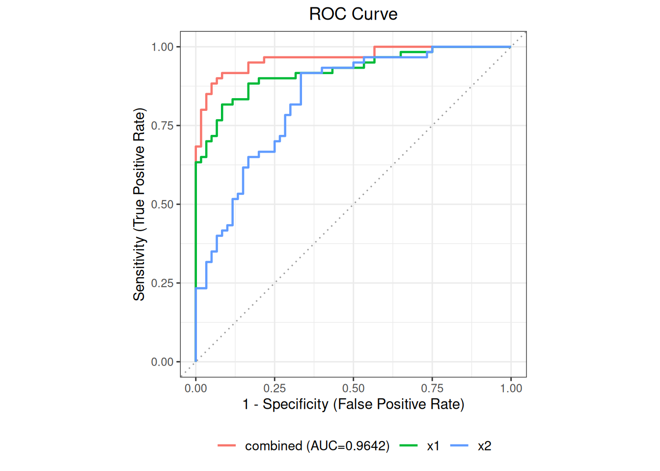

新样本预测与列名映射

代码

new_patients <- data.frame(
  x1 = c(7, 12),
  x2 = c(16, 21)
)
new_predictions <- predict(
  mlr_fit, mlr = "combined", newdata = new_patients
)
new_predictions

  x1 x2 pred_prob    pred_se   ci_lower  ci_upper pred_class
1  7 16 0.1200103 0.05313595 0.04840777 0.2677265          0
2 12 21 0.9781557 0.01751040 0.89984790 0.9955390          1

两例预测概率分别为 0.1200 和 0.9782，按内置 0.5 阈值分别显示为 0 和 1。区间反映拟合平均概率的参数不确定性，不包含新个体结局本身的二项随机性，也不包含模型错误和人群迁移。

新数据列名不同时，映射方向是“新列名 = 训练列名”：

代码

renamed_patients <- data.frame(
  marker_a = c(7, 12),
  marker_b = c(16, 21)
)
mapped_predictions <- predict(
  mlr_fit,
  mlr = "combined",
  newdata = renamed_patients,
  column_map = c(marker_a = "x1", marker_b = "x2")
)

12.2.2 CLSI EP24-A2 附录 D：两条配对 ROC

EP24 附录 D 的 OxLDL 和 LDL 都来自同一组 50 名受试者，因此两条 AUC 相关。先在同一个 roc 对象中计算两条经验 AUC 及单曲线 Hanley–McNeil 区间，再调用 auc_compare()；函数由共同完整病例保证配对关系。

代码

ep24_pair <- as.data.frame(read_csv(
  "./data/公共/std-ep24-appendix-d.csv",
  show_col_types = FALSE
))
ep24_pair_fit <- roc(
  ep24_pair, cols = c("oxldl", "ldl"),
  reference = "diagnosis", id = "id"
)
ep24_pair_fit <- auc(ep24_pair_fit)


AUC Table
  Column               AUC          95% CI  Direction
  ------------------------------------------------------------ 
  oxldl             0.7995  [0.6777, 0.9213]       geq
  ldl               0.5617  [0.4012, 0.7222]       geq

代码

ep24_pair_fit


ROC Analysis
  Data class:        data.frame
  Total rows:        50
  Complete cases:    50
  Reference:         diagnosis (binary)
  Reference coding:  binary (0/1)
  Positive / Neg:    28 / 22
  Evaluation cols:   2  (oxldl, ldl)
  Duplicate IDs:     none

Analysis slots:
    [ ] Describe
    [x] AUC
    [ ] Paired AUC comparison
    [ ] Cutoff
    [ ] MLR

默认的 EP24 方法按标准式（6）计算

\[ \operatorname{SE}(\widehat A_1-\widehat A_2) =\sqrt{\operatorname{SE}_1^2+\operatorname{SE}_2^2 -2r\operatorname{SE}_1\operatorname{SE}_2}, \]

其中 \(r\) 是由阳性、阴性组内评分相关的平均值和平均 AUC 对 EP24 表 5 插值得到的 AUC 相关。DeLong 方法不使用这项查表近似，而是通过每名阳性和阴性受试者的配对秩贡献估计协方差：

定义

\[ \phi(x,y)=I(x>y)+\frac12I(x=y), \]

对第 \(k\) 个标记物、\(m\) 个阳性和 \(n\) 个阴性，建立

\[ V_{10,i}^{(k)}=\frac1n\sum_{j=1}^{n}\phi(X_{ki},Y_{kj}), \qquad V_{01,j}^{(k)}=\frac1m\sum_{i=1}^{m}\phi(X_{ki},Y_{kj}). \]

两个标记物 AUC 向量的 DeLong 协方差估计为

\[ \widehat{\boldsymbol\Sigma} =\frac{\operatorname{Cov}(\mathbf V_{10})}{m} +\frac{\operatorname{Cov}(\mathbf V_{01})}{n}. \]

令 \(\mathbf c=(1,-1)^\mathsf T\)，则差值 \(\widehat\Delta=\widehat A_{\mathrm{OxLDL}}-\widehat A_{\mathrm{LDL}}\) 的标准误为

\[ \operatorname{SE}(\widehat\Delta) =\sqrt{\mathbf c^\mathsf T\widehat{\boldsymbol\Sigma}\mathbf c}. \]

代码

ep24_pair_fit <- auc_compare(
  ep24_pair_fit,
  curves = c("oxldl", "ldl"),
  method = "ep24"
)


Paired AUC Comparison
  Curves: oxldl - ldl
  Method: EP24-A2 Hanley-McNeil paired approximation
  Subjects: 50 (positive = 28, negative = 22)
  AUC oxldl: 0.799513
  AUC ldl: 0.561688
  Difference: 0.237825
  SE difference: 0.075261
  95.0% CI: [0.090315, 0.385334]
  z = 3.159979
  p-value: 0.0015778
  Mean within-group rating correlation: 0.511818
  EP24 area correlation: 0.481818
  Table lookup used bounded coordinates: correlation 0.5118, AUC 0.7000

把现场计算值与检查表中的 EP24 公布值比较：

EP24-A2 附录 D：单曲线和配对差异结果对照
标准位置	统计量	标准结果	ivdtools结果
OxLDL	AUC	0.8000	0.799513
OxLDL	SE	0.0620	0.062140
OxLDL	CI_lower	0.6800	0.677718
OxLDL	CI_upper	0.9200	0.921308
LDL	AUC	0.5600	0.561688
LDL	SE	0.0820	0.081895
LDL	CI_lower	0.4000	0.401174
LDL	CI_upper	0.7200	0.722203
Difference	AUC_difference	0.2400	0.237825
Difference	SE	0.0750	0.075261
Difference	CI_lower	0.0900	NA
Difference	CI_upper	0.3900	NA
Difference	z	3.1600	3.159979
Difference	p_value	0.0016	0.001578

12.1 主要函数

12.1.1 多元 Logistic 回归 mlr()

12.1.2 配对 AUC 比较 auc_compare()

12.1.3 概率预测 predict()