代码
library(ivdtools)
library(readr)方法学比较(method comparison)评价候选方法(candidate)与参考方法(reference)在相同样本上 测得结果的一致性,对应 CLSI EP09。ivdtools 的 mcr() 提供一个渐进式 S3 工作流:描述统计 → 相关分析 → 回归(OLS、WLS、Deming、加权 Deming、Passing–Bablok)→ Bland–Altman → 异常值 → 医学决定水平偏倚,并提供绘图、预测与汇总。本文以一个包含不同批次与样本类型的完整示例演示全流程, 并演示按批次/样本类型拆分后的子组比较。
示例数据为确定性的教学数据,其中人为加入了一个离群点以演示异常值检测;统计结果不自动构成合格 判定,接受标准应在分析前确定。
library(ivdtools)
library(readr)| 函数 | 主要用途 | 关键输入或输出 |
|---|---|---|
mcr() |
创建方法学比较对象 | id、candidate、reference、weights |
describe() |
描述统计 | 候选/参考/差值及额外列 |
correlation() |
相关分析 | pearson/spearman/kendall |
regression() |
回归拟合 | ols/wls/deming/wdeming/pb、lambda、weights |
bland_altman() |
一致性限 | difference/ratio/percent、x_axis |
outlier() |
差值异常值 | grubbs/esd/dixon/iqr、type |
bias() |
医学决定水平偏倚 | mdl、interval |
predict() |
正向/逆向预测 | 需先回归 |
plot() / summary() |
图形与汇总 | type 选择图形 |
数据包含 40 例,每例有编号 id、候选方法结果 candidate、参考方法结果 reference, 以及批次 batch(B1/B2)与样本类型 sample_type(serum/plasma/urine):
mc_dat <- read_csv("./data/method-comparison.csv", show_col_types = FALSE)
mc_dat <- as.data.frame(mc_dat)
str(mc_dat)
'data.frame': 40 obs. of 5 variables:
$ id : num 1 2 3 4 5 6 7 8 9 10 ...
$ batch : chr "B1" "B1" "B1" "B1" ...
$ sample_type: chr "serum" "plasma" "urine" "serum" ...
$ reference : num 10 14.9 19.7 24.6 29.5 34.4 39.2 44.1 49 53.8 ...
$ candidate : num 11.6 16.6 20.9 30.4 34 ...dim(mc_dat)[1] 40 5knitr::kable(table(mc_dat$batch), caption = "批次分布")| Var1 | Freq |
|---|---|
| B1 | 20 |
| B2 | 20 |
knitr::kable(table(mc_dat$sample_type), caption = "样本类型分布")| Var1 | Freq |
|---|---|
| plasma | 13 |
| serum | 14 |
| urine | 13 |
mc <- mcr(mc_dat, id = "id", candidate = "candidate", reference = "reference")mc <- describe(mc, cols = c("batch", "sample_type"))
Descriptive Statistics
  Variable               n     Mean       SD      Min       Q1   Median       Q3      Max  NA
  ---------------------------------------------------------------------------
    candidate (X)       40 112.4977  59.2513  11.5900  63.1075 112.5750 159.5925 209.9000
    reference (Y)       40 105.0000  56.9555  10.0000  57.4750 105.0000 152.5250 200.0000
    Diff (X-Y)          40   7.4977   3.9583   1.2000   5.2725   6.6100   9.7950  22.1000

  batch
  Level                Count  Percent
   --------------------------------------
  B1                      20    50.0%
  B2                      20    50.0%

  sample_type
  Level                Count  Percent
   --------------------------------------
  plasma                  13    32.5%
  serum                   14    35.0%
urine 13 32.5%mc
Method Comparison
  Data class:        data.frame
  Total rows:        40
  Complete pairs:    40
  ID variable:       id
  Test method (X):   candidate
  Reference (Y):     reference
  Duplicate IDs:     none

Analysis slots:
    [x] Describe
    [ ] Correlation
    [ ] Regression
    [ ] Outlier
    [ ] Bland-Altman
    [ ] Bias
describe() 的 cols 指定纳入描述的分类/数值附加列,支持 - 前缀排除。
mc <- correlation(mc, method = "pearson")
Correlation
  Method: pearson
  r = 0.9985, 95% CI [0.9971, 0.9992]
  p-value: < 2.2e-16
  n = 40
参数说明:
correlation()的method可选"pearson"、"spearman"、"kendall"。 相关反映两变量共同变化的程度,不等于一致性,不能替代 Bland–Altman 或回归偏差评价。
依次比较 OLS、Deming、Passing–Bablok 与 WLS。由于 regression() 会更新对象内的回归结果,多种 方法分别存入不同对象以便比较:
mc_ols <- regression(mc, method = "ols")
Regression
  Method: OLS
  Intercept = -2.9723  (SE = 1.0971)
  Slope     = 0.9598  (SE = 0.0087)
  Intercept 95% CI: [-5.1933, -0.7513]
  Slope     95% CI: [0.9423, 0.9773]
    H0: slope = 1 -> t = -4.6494, p = 3.944e-05
    slope significantly different from 1 (CI excludes 1)
  R-squared = 0.9969
  Sigma     = 3.2015
n = 40mc_dem <- regression(mc, method = "deming")
Regression
  Method: Deming
  Intercept = -3.1323  (SE = 1.4133)
  Slope     = 0.9612  (SE = 0.0092)
  Intercept 95% CI: [-5.9934, -0.2712]
  Slope     95% CI: [0.9426, 0.9798]
    H0: slope = 1 -> t = -4.2313, p = 0.0001413
    slope significantly different from 1 (CI excludes 1)
  Sigma     = 3.2026
n = 40mc_pb <- regression(mc, method = "pb")
Regression
  Method: Passing-Bablok
  Intercept = -2.1674  (SE =    NA)
  Slope     = 0.9556  (SE =    NA)
  Intercept 95% CI: [-3.1487, -0.9828]
  Slope     95% CI: [0.9444, 0.9669]
  Sigma     = 3.2299
n = 40mc_wls <- regression(mc, method = "wls", weights = "1/y")
Regression
  Method: WLS
  Weights: 1/y
  Intercept = -2.2924  (SE = 0.9153)
  Slope     = 0.9518  (SE = 0.0108)
  Intercept 95% CI: [-4.1452, -0.4396]
  Slope     95% CI: [0.9299, 0.9736]
    H0: slope = 1 -> t = -4.4712, p = 6.818e-05
    slope significantly different from 1 (CI excludes 1)
  R-squared = 0.9951
  Sigma     = 0.4819
n = 40knitr::kable(
data.frame(
方法 = c("OLS", "Deming", "Passing-Bablok", "WLS(1/y)"),
截距 = c(mc_ols$regression$intercept, mc_dem$regression$intercept,
mc_pb$regression$intercept, mc_wls$regression$intercept),
斜率 = c(mc_ols$regression$slope, mc_dem$regression$slope,
mc_pb$regression$slope, mc_wls$regression$slope)
),
digits = 4,
caption = "四种回归方法截距与斜率比较"
)| 方法 | 截距 | 斜率 |
|---|---|---|
| OLS | -2.9723 | 0.9598 |
| Deming | -3.1323 | 0.9612 |
| Passing-Bablok | -2.1674 | 0.9556 |
| WLS(1/y) | -2.2924 | 0.9518 |
print(mc_ols)
Method Comparison
  Data class:        data.frame
  Total rows:        40
  Complete pairs:    40
  ID variable:       id
  Test method (X):   candidate
  Reference (Y):     reference
  Duplicate IDs:     none

Analysis slots:
    [x] Describe
    [x] Correlation (pearson)
    [x] Regression (OLS)
    [ ] Outlier
    [ ] Bland-Altman
    [ ] Bias
本例 OLS 斜率 ≈ 0.96,95% CI 不含 1,说明候选方法存在约 4% 的比例偏差(数据真实偏差即为 5%)。
参数说明:
regression()的method可选"ols"、"wls"、"deming"、"wdeming"、"pb"。 Deming 用lambda指定方差比(ref/cand,默认 1);wls/wdeming必须提供weights(内置方案 或数据列名);conf.level控制参数置信区间。
用 bias() 评价在医学决定水平(MDL)处的预测偏倚:
mc_ols <- bias(mc_ols, mdl = c(30, 80, 150), interval = "both")
Bias
  Method: OLS
  Interval: both (95%)
  MDL points: 3
  Bias range: [4.1791, 9.0064]

 mdl     bias ci_lower  ci_upper  pi_lower pi_upper
---------------------------------------------------
  30 4.179112 2.407658  5.950566 -2.539698 10.89792
  80 6.190463 5.018240  7.362685 -0.395770 12.77670
150 9.006354 7.789153 10.223554 2.411967 15.60074 mc_ols$biasplot(mc_ols, type = "bias", mdl = c(30, 80, 150))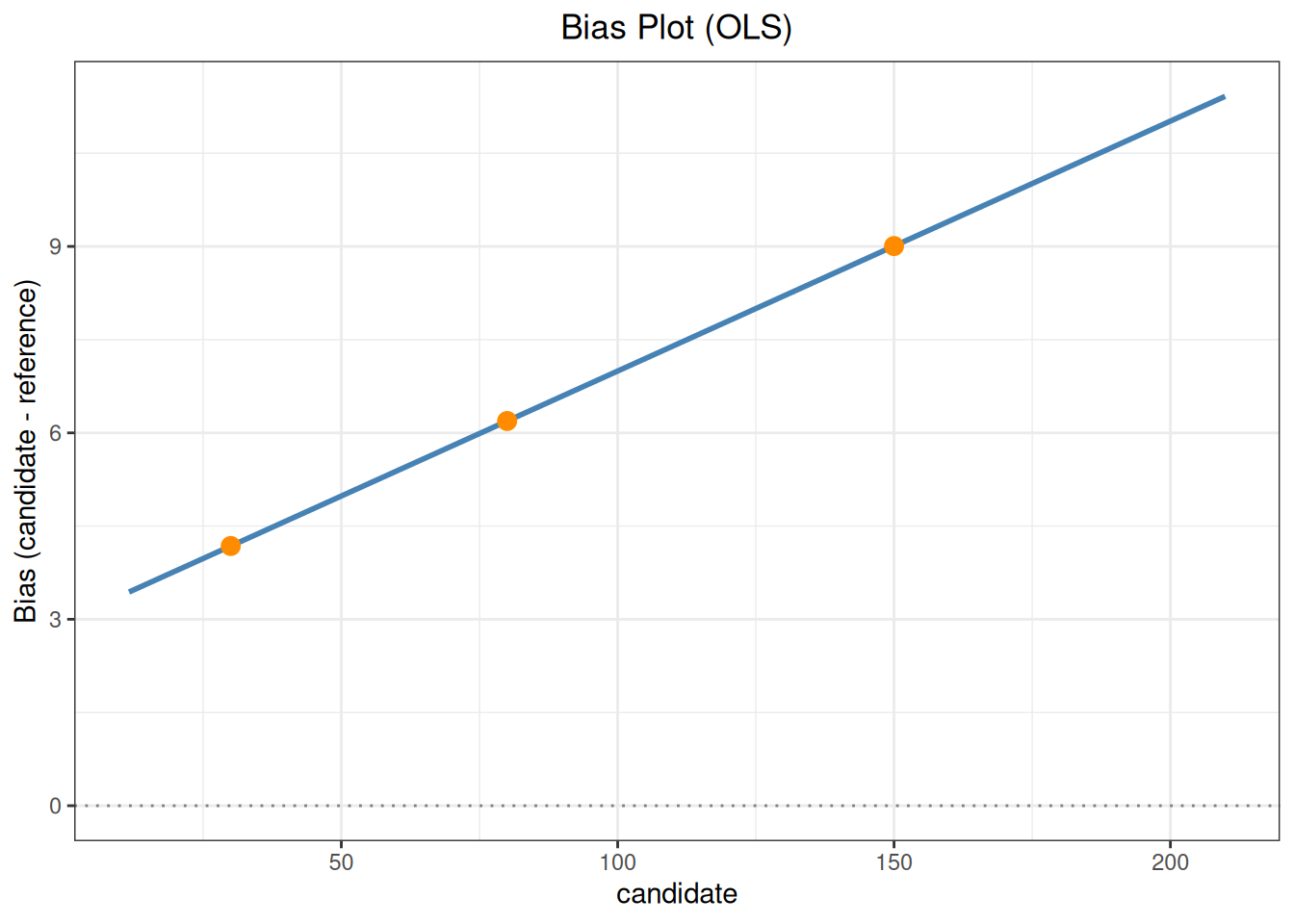
参数说明:
bias(mdl, level, interval)中mdl为医学决定水平向量;interval可选""、"confidence"、"prediction"、"both"。偏倚定义参考候选方法mdl处的拟合值与mdl之差,解释时应结合回归方向和方案规定的允许偏倚。
mc_ols <- bland_altman(mc_ols, type = "difference")
Bland-Altman
  Type:        difference
  Y-axis:      candidate - reference
  X-axis:      Mean of candidate and reference
  n = 40

  Mean diff:       7.4977
  SD diff:         3.9583
  95% LoA: [-0.2603, 15.2558]

  95% CI for LoA:
    Lower LoA: [-2.4419, 1.9213]
Upper LoA: [13.0742, 17.4374]plot(mc_ols, type = "bland_altman")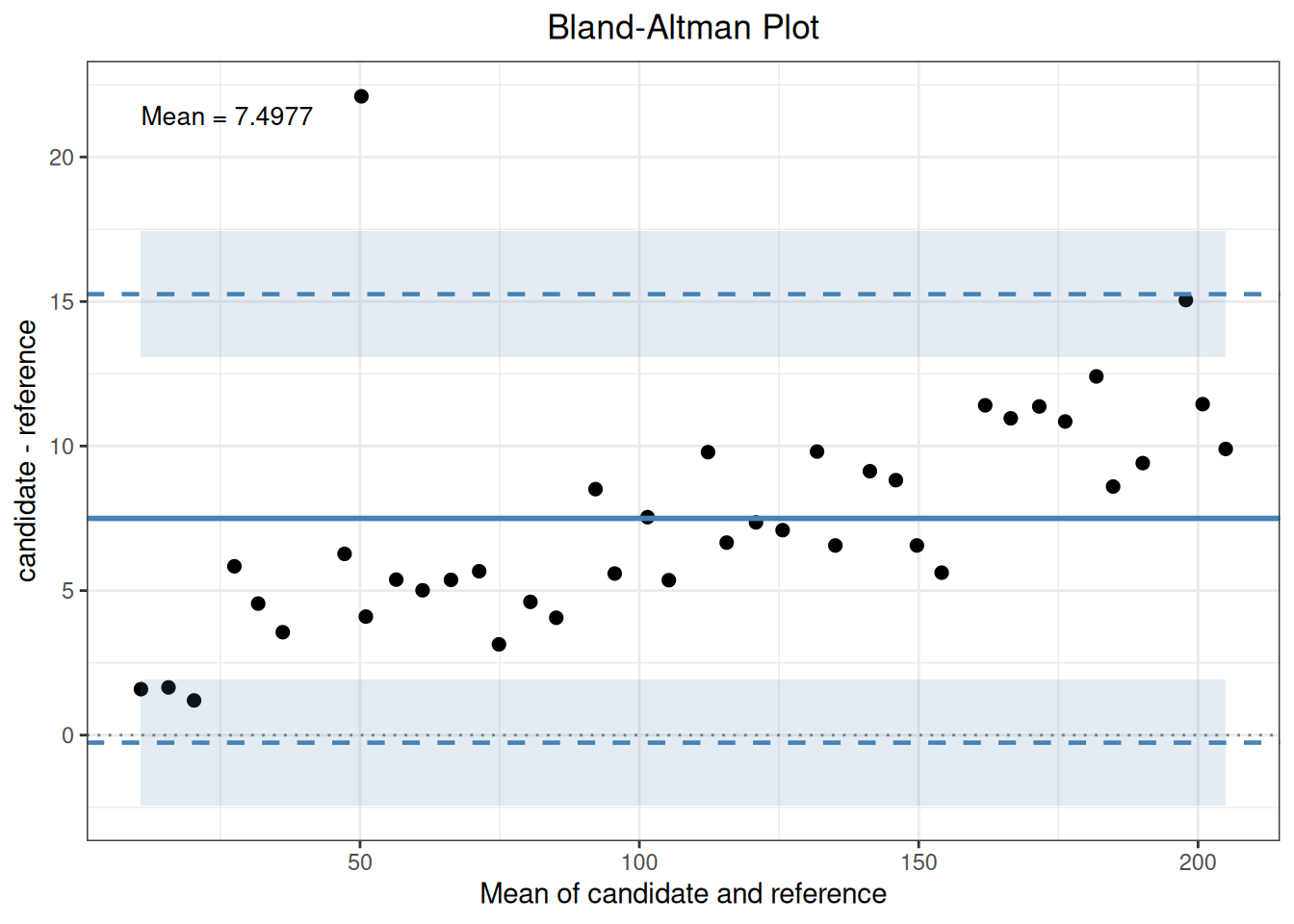
mc_ols$bland_altman[c("mean_diff", "sd_diff", "loa")]$mean_diff
[1] 7.49775
$sd_diff
[1] 3.958259
$loa
lower upper
-0.2602947 15.2557947 参数说明:
bland_altman()的type可选"difference"、"ratio"、"percent"(Y 轴度量),x_axis可选"mean"、"candidate"、"reference"(X 轴);agree.level控制 LoA 宽度,conf.level控制 LoA 置信区间。
对配对差值检测异常值:
mc_ols <- outlier(mc_ols, method = "grubbs", type = "difference")
Outlier
  Method: grubbs
  Data:   Difference (candidate - reference)
  Alpha:  0.05

  1 outlier(s) found:
  Row                Value   Statistic  Critical
   --------------------------------------------------
7 22.1000 3.6891 3.0361mc_ols$outlier
Outlier
  Method: grubbs
  Data:   Difference (candidate - reference)
  Alpha:  0.05

  1 outlier(s) found:
  Row                Value   Statistic  Critical
   --------------------------------------------------
7 22.1000 3.6891 3.0361mc_ols$outlier$indices[1] 7检测到第 7 号样本的差值明显偏大。检出异常值不等于应删除——应回查原始记录、实验过程,并在有 充分理由时进行包含/不包含的敏感性分析。
predict(mc_ols, candidate = c(40, 100))predict(mc_ols, reference = c(50, 120), inverse = TRUE)不同批次或样本类型的方法表现可能不同。先按批次拆分,再对子组重跑回归与 Bland–Altman:
for (b in c("B1", "B2")) {
  sub <- mc_dat[mc_dat$batch == b, ]
  mcs <- mcr(sub, id = "id", candidate = "candidate", reference = "reference")
  mcs <- regression(mcs, method = "ols")
  mcs <- bland_altman(mcs, type = "difference")
  cat(b, ": slope =", round(mcs$regression$slope, 4),
      ", mean diff =", round(mcs$bland_altman$mean_diff, 3), "\n")
}
Regression
  Method: OLS
  Intercept = -2.9704  (SE = 2.2333)
  Slope     = 0.9582  (SE = 0.0327)
  Intercept 95% CI: [-7.6623, 1.7215]
  Slope     95% CI: [0.8895, 1.0269]
    H0: slope = 1 -> t = -1.2784, p = 0.2173
    slope not significantly different from 1 (CI contains 1)
  R-squared = 0.9795
  Sigma     = 4.2427
  n = 20

Bland-Altman
  Type:        difference
  Y-axis:      candidate - reference
  X-axis:      Mean of candidate and reference
  n = 20

  Mean diff:       5.5550
  SD diff:         4.3129
  95% LoA: [-2.8981, 14.0081]

  95% CI for LoA:
    Lower LoA: [-6.4069, 0.6107]
    Upper LoA: [10.4993, 17.5169]
B1 : slope = 0.9582 , mean diff = 5.555

Regression
  Method: OLS
  Intercept = -1.3159  (SE = 2.3598)
  Slope     = 0.9502  (SE = 0.0142)
  Intercept 95% CI: [-6.2736, 3.6419]
  Slope     95% CI: [0.9203, 0.9801]
    H0: slope = 1 -> t = -3.4988, p = 0.002564
    slope significantly different from 1 (CI excludes 1)
  R-squared = 0.9960
  Sigma     = 1.8780
  n = 20

Bland-Altman
  Type:        difference
  Y-axis:      candidate - reference
  X-axis:      Mean of candidate and reference
  n = 20

  Mean diff:       9.4405
  SD diff:         2.3693
  95% LoA: [4.7968, 14.0842]

  95% CI for LoA:
    Lower LoA: [2.8693, 6.7244]
    Upper LoA: [12.1566, 16.0117]
B2 : slope = 0.9502 , mean diff = 9.44
按样本类型同理 split() 后分别分析。子组比较的结论用于判断方法表现是否受批次/样本类型影响, 只有预先定义的接受标准才能支撑可接受性结论。
summary(mc_ols)
Method Comparison Regression (mcr)
-----------------------------------------------------

Method Comparison
  Data class:        data.frame
  Total rows:        40
  Complete pairs:    40
  ID variable:       id
  Test method (X):   candidate
  Reference (Y):     reference
  Duplicate IDs:     none

Analysis slots:
    [x] Describe
    [x] Correlation (pearson)
    [x] Regression (OLS)
    [x] Outlier (grubbs)
    [x] Bland-Altman (difference)
    [x] Bias

Descriptive Statistics
  Variable               n     Mean       SD      Min       Q1   Median       Q3      Max  NA
  ---------------------------------------------------------------------------
    candidate (X)       40 112.4977  59.2513  11.5900  63.1075 112.5750 159.5925 209.9000
    reference (Y)       40 105.0000  56.9555  10.0000  57.4750 105.0000 152.5250 200.0000
    Diff (X-Y)          40   7.4977   3.9583   1.2000   5.2725   6.6100   9.7950  22.1000

  batch
  Level                Count  Percent
   --------------------------------------
  B1                      20    50.0%
  B2                      20    50.0%

  sample_type
  Level                Count  Percent
   --------------------------------------
  plasma                  13    32.5%
  serum                   14    35.0%
  urine                   13    32.5%

Correlation
  Method: pearson
  r = 0.9985, 95% CI [0.9971, 0.9992]
  p-value: < 2.2e-16
  n = 40

Regression
  Method: OLS
  Intercept = -2.9723  (SE = 1.0971)
  Slope     = 0.9598  (SE = 0.0087)
  Intercept 95% CI: [-5.1933, -0.7513]
  Slope     95% CI: [0.9423, 0.9773]
    H0: slope = 1 -> t = -4.6494, p = 3.944e-05
    slope significantly different from 1 (CI excludes 1)
  R-squared = 0.9969
  Sigma     = 3.2015
  n = 40

Outlier
  Method: grubbs
  Data:   Difference (candidate - reference)
  Alpha:  0.05

  1 outlier(s) found:
  Row                Value   Statistic  Critical
   --------------------------------------------------
  7                22.1000      3.6891  3.0361

Bland-Altman
  Type:        difference
  Y-axis:      candidate - reference
  X-axis:      Mean of candidate and reference
  n = 40

  Mean diff:       7.4977
  SD diff:         3.9583
  95% LoA: [-0.2603, 15.2558]

  95% CI for LoA:
    Lower LoA: [-2.4419, 1.9213]
    Upper LoA: [13.0742, 17.4374]

Bias
  Method: OLS
  Interval: both (95%)
  MDL points: 3
  Bias range: [4.1791, 9.0064]

 mdl     bias ci_lower  ci_upper  pi_lower pi_upper
---------------------------------------------------
  30 4.179112 2.407658  5.950566 -2.539698 10.89792
  80 6.190463 5.018240  7.362685 -0.395770 12.77670
 150 9.006354 7.789153 10.223554  2.411967 15.60074